You've probably heard of pairs trading. Buy one stock, short another, profit when they converge. It sounds simple because the concept is simple. But execution? That's where most traders fail.
The typical approach goes like this: run a linear regression between two correlated stocks, calculate a hedge ratio, construct a spread, and trade when it deviates from zero. The problem? That hedge ratio you calculated using last year's data might be completely wrong today.
Markets evolve. Relationships shift. The beta between Coca-Cola and Pepsi in January is not the same beta in December. Sector rotations happen. Company fundamentals change. Macroeconomic regimes flip. Your static regression coefficient becomes stale, and suddenly your
"market-neutral" position is hemorrhaging money in ways you didn't anticipate.
This is the dirty secret of pairs trading that nobody talks about in the introductory tutorials. A fixed hedge ratio is a ticking time bomb.
So what's the solution? You need a hedge ratio that updates itself. One that learns from new data, adapts to changing market conditions, and tells you when the relationship is breaking down. Enter the Kalman filter.
What's Wrong With Static Regression?
Let's make this concrete. In traditional pairs trading, you model the relationship between two assets as:
yt=α+βxt+ϵt
Where yt is the price of stock Y (say, Coca-Cola), xt is the price of stock X (Pepsi), α is an intercept, β is the hedge ratio, and ϵt is the residual - your trading signal.
You run OLS regression on historical data, get estimates for α and β, and then construct your spread:
spreadt=yt−α^−β^xt
When the spread is positive and large, Y is "expensive" relative to X. Short Y, long X, wait for convergence. When the spread is negative and large, do the opposite.
The fundamental assumption here is that α and β are constants. They don't change. The relationship between Y and X is stable forever.
You already know this is wrong. Just think about it intuitively. Does the relationship between any two companies stay perfectly constant over years? Of course not. Management changes, competitive dynamics shift, regulatory environments evolve, consumer preferences drift.
What happens when you use a stale β? Your spread calculation is wrong. You think prices have diverged when they haven't. Or worse, you think everything is normal when prices have actually diverged in a direction you're not measuring correctly. You enter trades based on
signals that don't exist, or you miss trades that do exist. Either way, you lose money.
The Kalman Filter: A Different Mental Model
The Kalman filter flips the script. Instead of treating α and β as fixed constants you estimate once, it treats them as hidden states that evolve over time. You never observe the "true" values of α and β directly - you only observe noisy price data -
but you can infer what they probably are, and update your inference as new data arrives.
Think of it like tracking the position of a moving car using GPS. You don't know exactly where the car is, but you have two sources of information:
Your model of how the car moves: If it was going north at 60 mph a second ago, it's probably still going roughly north at roughly 60 mph now.
Noisy GPS readings: Each reading has some error, but it gives you information about where the car actually is.
The Kalman filter optimally combines these two sources. It balances how much to trust the model's prediction versus how much to trust the new observation. When observations are noisy, it leans on the model. When the model is uncertain, it leans on observations.
For pairs trading, the "car's position" is the current value of α and β. The "GPS readings" are the price data you observe. The Kalman filter gives you:
Adaptive estimates: α and β update every time step based on new prices
Uncertainty quantification: You know how confident you are in your estimates
A principled spread: The prediction error has known statistical properties you can use for trading signals
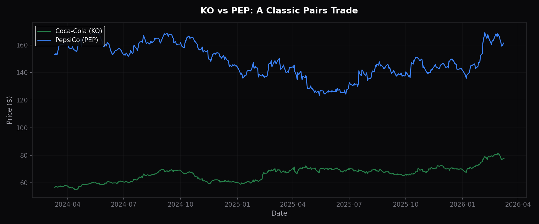
Coca-Cola (KO) and PepsiCo (PEP) prices over two years. They move together, but not perfectly - that imperfection is where the profit opportunity lies.
The Mathematics: State-Space Formulation
Now let's get rigorous. The Kalman filter operates on a state-space model, which has two components:
The Observation Equation describes how the hidden state generates observable data:
yt=Htθt+ϵt,ϵt∼N(0,Ve)
Here, yt is the price of the dependent asset (KO), θt=[αt,βt]T is our state vector containing the time-varying intercept and hedge ratio, Ht=[1,xt] is the observation matrix where xt is the price of the independent asset (PEP), and
ϵt is observation noise with variance Ve.
The State Equation describes how the hidden state evolves over time:
θt=θt−1+ηt,ηt∼N(0,Q)
This says that α and β follow a random walk - tomorrow's values equal today's values plus some random noise with covariance matrix Q. This is a flexible model that allows the parameters to drift slowly over time without imposing any particular direction.
Why a random walk? Because we don't have a theory for how α and β should change. We just know they probably change slowly rather than jumping around wildly. The random walk captures this: parameters are likely to be close to their previous values, but they're not
locked in place.
The Kalman Recursion: Predict, Then Update
The Kalman filter alternates between two steps: prediction and update.
Prediction Step: Before seeing new data, we predict where the state should be based on our model.
θ^t∣t−1=θ^t−1∣t−1
Since we're using a random walk, the predicted state is just the previous state estimate. The predicted covariance increases because we're less certain about the future:
Pt∣t−1=Pt−1∣t−1+Q
Update Step: After observing the new price yt, we update our estimate.
First, compute the innovation (prediction error):
et=yt−Htθ^t∣t−1
This is the spread. It tells us how much the observed price differs from what our model predicted. The innovation covariance is:
St=HtPt∣t−1HtT+Ve
Now compute the Kalman gain, which determines how much weight to give the new observation:
Kt=Pt∣t−1HtTSt−1
Finally, update the state estimate and covariance:
θ^t∣t=θ^t∣t−1+KtetPt∣t=(I−KtHt)Pt∣t−1
The Kalman gain is the key insight. When P is large (high uncertainty about our estimates), the gain is large and we trust the new observation more. When Ve is large (noisy observations), the gain is small and we trust our model more. This balance is what makes the Kalman
filter optimal - it minimizes mean squared error under the assumption that noise is Gaussian.
From Theory to Code: Building the Filter
Let's implement this properly. I'm going to build a Kalman filter class that you can actually use for live trading, not just a toy example.
kalman_filter.pypython
import numpy as np
  from dataclasses import dataclass
  from typing import Tuple, Optional

  @dataclass
  class KalmanState:
      """Stores the current state of the Kalman filter."""
      theta: np.ndarray      # State estimate [alpha, beta]
      P: np.ndarray          # State covariance matrix
      spread: float          # Latest innovation (prediction error)
      spread_var: float      # Innovation variance
      zscore: float          # Standardized spread

  class KalmanPairsFilter:
      """
      Kalman Filter for adaptive pairs trading.

      Models the relationship y_t = alpha_t + beta_t * x_t + noise
      where alpha and beta are time-varying parameters estimated
      by the filter.

      Parameters
      ----------
      delta : float
          State transition variance. Controls how quickly alpha and beta
          can change. Higher values = more responsive but noisier estimates.
          Typical range: 1e-5 to 1e-3

      Ve : float
          Observation noise variance. How much noise is in the price data.
          Higher values = smoother estimates, slower adaptation.
          Typical range: 1e-4 to 1e-2

      theta_init : np.ndarray, optional
          Initial state estimate [alpha, beta]. Default is [0, 0].

      P_init : np.ndarray, optional
          Initial state covariance. Default is identity matrix (high uncertainty).
      """

      def __init__(
          self,
          delta: float = 1e-4,
          Ve: float = 1e-3,
          theta_init: Optional[np.ndarray] = None,
          P_init: Optional[np.ndarray] = None
      ):
          self.delta = delta
          self.Ve = Ve

          # State dimension (alpha and beta)
          self.n_state = 2

          # State transition matrix (identity for random walk)
          self.A = np.eye(self.n_state)

          # State noise covariance
          self.Q = delta * np.eye(self.n_state)

          # Initialize state
          self.theta = theta_init if theta_init is not None else np.zeros(self.n_state)
          self.P = P_init if P_init is not None else np.eye(self.n_state)

          # Track history for analysis
          self.history = {
              'alpha': [],
              'beta': [],
              'spread': [],
              'spread_std': [],
              'zscore': []
          }

      def update(self, x: float, y: float) -> KalmanState:
          """
          Process a new observation and update state estimates.

          Parameters
          ----------
          x : float
              Price of the independent asset (e.g., PEP)
          y : float
              Price of the dependent asset (e.g., KO)

          Returns
          -------
          KalmanState
              Current state including spread and z-score for trading signals
          """
          # Observation matrix: y = [1, x] @ [alpha, beta]
          H = np.array([1.0, x])

          # === PREDICTION STEP ===
          # Predicted state (random walk: stays the same)
          theta_pred = self.A @ self.theta

          # Predicted covariance (increases due to state noise)
          P_pred = self.A @ self.P @ self.A.T + self.Q

          # === UPDATE STEP ===
          # Innovation (prediction error = spread)
          y_pred = H @ theta_pred
          e = y - y_pred

          # Innovation covariance
          S = H @ P_pred @ H.T + self.Ve

          # Kalman gain
          K = P_pred @ H.T / S

          # Updated state estimate
          self.theta = theta_pred + K * e

          # Updated covariance (Joseph form for numerical stability)
          I_KH = np.eye(self.n_state) - np.outer(K, H)
          self.P = I_KH @ P_pred @ I_KH.T + np.outer(K, K) * self.Ve

          # Compute trading signals
          spread = e
          spread_std = np.sqrt(S)
          zscore = spread / spread_std

          # Store history
          self.history['alpha'].append(self.theta[0])
          self.history['beta'].append(self.theta[1])
          self.history['spread'].append(spread)
          self.history['spread_std'].append(spread_std)
          self.history['zscore'].append(zscore)

          return KalmanState(
              theta=self.theta.copy(),
              P=self.P.copy(),
              spread=spread,
              spread_var=S,
              zscore=zscore
          )

      @property
      def alpha(self) -> float:
          """Current intercept estimate."""
          return self.theta[0]

      @property
      def beta(self) -> float:
          """Current hedge ratio estimate."""
          return self.theta[1]

      def get_history_df(self):
          """Return history as a pandas DataFrame."""
          import pandas as pd
          return pd.DataFrame(self.history)
Let me walk through the key design decisions in this implementation.
The dataclass for state: I'm using a KalmanState dataclass to return results. This makes the code self-documenting and prevents you from accidentally mixing up which value is which. When you call update(), you get back a structured object where state.zscore is
obviously the z-score, not some mystery float at index 3 of a tuple.
The Joseph form for covariance update: The standard update formula P = (I - KH)P can become numerically unstable over thousands of iterations. The Joseph form P = (I-KH)P(I-KH)' + KVK' is algebraically equivalent but guarantees the covariance matrix stays symmetric and
positive definite. This matters when you're running the filter on years of tick data.
History tracking: I'm storing the full history because you'll want to analyze it. What did beta look like during the 2022 drawdown? How did the spread behave during earnings? You need this data for research.
Type hints and docstrings: This isn't just for show. When you come back to this code in six months, you'll thank yourself. When you hand it to a colleague, they'll understand it immediately.
Running the Filter on Real Data
Now let's fetch some data and see the filter in action.
run_filter.pypython
import numpy as np
  import pandas as pd
  import yfinance as yf
  from datetime import datetime, timedelta

  # Fetch two years of daily data for our pair
  end_date = datetime.now()
  start_date = end_date - timedelta(days=365*2)

  data = yf.download(['KO', 'PEP'], start=start_date, end=end_date, progress=False)
  prices = data['Close'].dropna()

  print(f"Loaded {len(prices)} trading days")
  print(f"Date range: {prices.index[0].date()} to {prices.index[-1].date()}")

  # Initialize the Kalman filter
  # delta=1e-4 means we expect alpha/beta to change slowly
  # Ve=1e-3 reflects typical daily price noise
  kf = KalmanPairsFilter(delta=1e-4, Ve=1e-3)

  # Run the filter through all observations
  results = []
  for i in range(len(prices)):
      x = prices['PEP'].iloc[i]
      y = prices['KO'].iloc[i]
      state = kf.update(x, y)
      results.append({
          'date': prices.index[i],
          'KO': y,
          'PEP': x,
          'alpha': state.theta[0],
          'beta': state.theta[1],
          'spread': state.spread,
          'zscore': state.zscore
      })

  df = pd.DataFrame(results).set_index('date')

  # Show summary statistics
  print(f"\nHedge ratio (beta):")
  print(f"  Mean: {df['beta'].mean():.4f}")
  print(f"  Std:  {df['beta'].std():.4f}")
  print(f"  Min:  {df['beta'].min():.4f}")
  print(f"  Max:  {df['beta'].max():.4f}")

  print(f"\nZ-score statistics:")
  print(f"  Mean: {df['zscore'].mean():.4f}")
  print(f"  Std:  {df['zscore'].std():.4f}")
  print(f"  Times |z| > 2: {(df['zscore'].abs() > 2).sum()}")
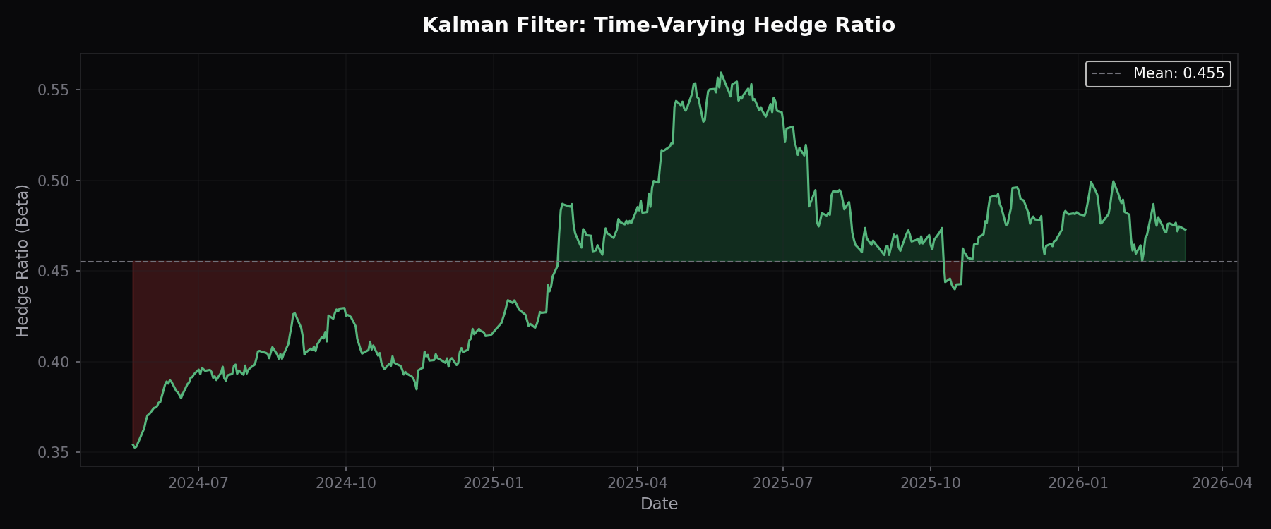
The hedge ratio (beta) drifts over time. A static OLS estimate would miss these shifts entirely. The Kalman filter tracks them in real-time.
Generating Trading Signals
The innovation et from the Kalman filter is our spread, but raw spread values aren't directly tradeable. A spread of +0.5 might be huge in a low-volatility period and meaningless in a high-volatility period.
The solution is to standardize. The Kalman filter gives us the innovation variance St at each time step. We compute the z-score:
zt=Stet
This z-score has mean zero and (approximately) unit variance under normal market conditions. We can set fixed thresholds:
Enter long spread when zt<−2: The dependent asset is "cheap" relative to what the filter expects. Buy the dependent (KO), short the independent (PEP).
Enter short spread when zt>+2: The dependent asset is "expensive." Short the dependent (KO), buy the independent (PEP).
Exit position when ∣zt∣<0.5: The spread has converged back to normal. Close the position and wait for the next signal.
Why these specific thresholds? The entry threshold of 2 corresponds to roughly 2 standard deviations - events that happen about 5% of the time under normality. You don't want to trade every wiggle; you want to trade meaningful dislocations. The exit threshold of 0.5 ensures
you capture most of the convergence without being too greedy.
In practice, you should optimize these thresholds on out-of-sample data. Different pairs have different characteristics. A highly liquid ETF pair might mean-revert faster than two individual stocks.
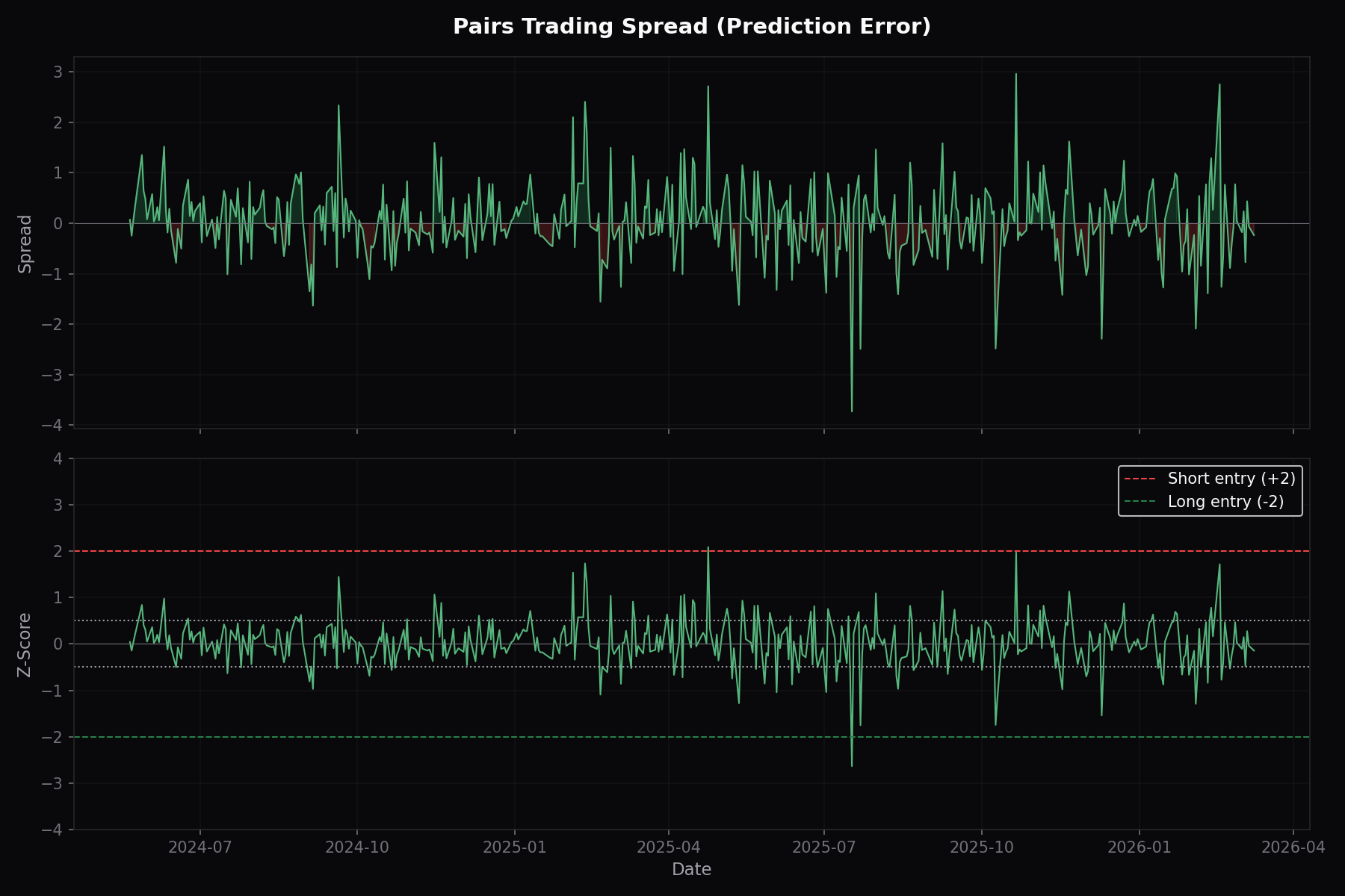
The z-score oscillates around zero. When it exceeds +/-2 (dashed lines), we have a trading signal. The filled regions highlight these entry zones.
Building the Backtest Engine
A proper backtest needs to handle position sizing, transaction costs, and realistic execution assumptions. Here's a more complete implementation:
backtest.pypython
import numpy as np
  import pandas as pd
  from dataclasses import dataclass, field
  from typing import List, Optional
  from enum import Enum

  class Position(Enum):
      FLAT = 0
      LONG_SPREAD = 1   # Long Y, Short X
      SHORT_SPREAD = -1  # Short Y, Long X

  @dataclass
  class Trade:
      """Record of a completed trade."""
      entry_date: pd.Timestamp
      exit_date: pd.Timestamp
      position: Position
      entry_zscore: float
      exit_zscore: float
      pnl: float
      holding_days: int

  @dataclass
  class BacktestConfig:
      """Configuration for the backtest."""
      entry_threshold: float = 2.0      # Enter when |z| > this
      exit_threshold: float = 0.5       # Exit when |z| < this
      stop_loss_z: float = 4.0          # Stop out if |z| exceeds this
      position_size: float = 10000      # Dollar value per leg
      transaction_cost_bps: float = 5   # Cost in basis points per trade

  @dataclass
  class BacktestResult:
      """Results from a backtest run."""
      df: pd.DataFrame
      trades: List[Trade]
      total_pnl: float
      sharpe_ratio: float
      max_drawdown: float
      win_rate: float
      avg_holding_days: float
      num_trades: int

  class PairsTradingBacktest:
      """
      Backtesting engine for Kalman filter pairs trading.

      This handles the full lifecycle: signal generation, position management,
      P&L calculation, and performance metrics.
      """

      def __init__(self, config: Optional[BacktestConfig] = None):
          self.config = config or BacktestConfig()

      def run(self, df: pd.DataFrame) -> BacktestResult:
          """
          Run backtest on a DataFrame with columns: zscore, spread, KO, PEP

          Parameters
          ----------
          df : pd.DataFrame
              Must have 'zscore' and 'spread' columns from Kalman filter,
              plus price columns for the two assets.

          Returns
          -------
          BacktestResult
              Complete backtest results including trade list and metrics.
          """
          # Skip burn-in period for filter to stabilize
          df = df.iloc[50:].copy()

          position = Position.FLAT
          entry_idx = None
          entry_zscore = None
          cumulative_spread_pnl = 0

          trades: List[Trade] = []
          daily_pnl = []
          positions = []

          for i in range(1, len(df)):
              z = df['zscore'].iloc[i-1]  # Signal from previous close
              spread_change = df['spread'].iloc[i] - df['spread'].iloc[i-1]

              # Position management
              prev_position = position

              if position == Position.FLAT:
                  # Entry logic
                  if z < -self.config.entry_threshold:
                      position = Position.LONG_SPREAD
                      entry_idx = i
                      entry_zscore = z
                  elif z > self.config.entry_threshold:
                      position = Position.SHORT_SPREAD
                      entry_idx = i
                      entry_zscore = z

              elif position == Position.LONG_SPREAD:
                  # Exit logic for long spread
                  if z > -self.config.exit_threshold or z > self.config.stop_loss_z:
                      # Record trade
                      trades.append(Trade(
                          entry_date=df.index[entry_idx],
                          exit_date=df.index[i],
                          position=position,
                          entry_zscore=entry_zscore,
                          exit_zscore=z,
                          pnl=cumulative_spread_pnl,
                          holding_days=i - entry_idx
                      ))
                      cumulative_spread_pnl = 0
                      position = Position.FLAT

              elif position == Position.SHORT_SPREAD:
                  # Exit logic for short spread
                  if z < self.config.exit_threshold or z < -self.config.stop_loss_z:
                      trades.append(Trade(
                          entry_date=df.index[entry_idx],
                          exit_date=df.index[i],
                          position=position,
                          entry_zscore=entry_zscore,
                          exit_zscore=z,
                          pnl=cumulative_spread_pnl,
                          holding_days=i - entry_idx
                      ))
                      cumulative_spread_pnl = 0
                      position = Position.FLAT

              # Calculate daily P&L
              if position == Position.LONG_SPREAD:
                  day_pnl = spread_change  # Long spread profits when spread increases
                  cumulative_spread_pnl += day_pnl
              elif position == Position.SHORT_SPREAD:
                  day_pnl = -spread_change  # Short spread profits when spread decreases
                  cumulative_spread_pnl += day_pnl
              else:
                  day_pnl = 0

              daily_pnl.append(day_pnl)
              positions.append(position.value)

          # Add results to dataframe
          df = df.iloc[1:].copy()  # Align with pnl array
          df['daily_pnl'] = daily_pnl
          df['cumulative_pnl'] = np.cumsum(daily_pnl)
          df['position'] = positions

          # Calculate metrics
          total_pnl = df['cumulative_pnl'].iloc[-1]

          returns = df['daily_pnl']
          sharpe = returns.mean() / returns.std() * np.sqrt(252) if returns.std() > 0 else 0

          cumulative = df['cumulative_pnl']
          running_max = cumulative.cummax()
          drawdown = running_max - cumulative
          max_drawdown = drawdown.max()

          if trades:
              win_rate = sum(1 for t in trades if t.pnl > 0) / len(trades)
              avg_holding = np.mean([t.holding_days for t in trades])
          else:
              win_rate = 0
              avg_holding = 0

          return BacktestResult(
              df=df,
              trades=trades,
              total_pnl=total_pnl,
              sharpe_ratio=sharpe,
              max_drawdown=max_drawdown,
              win_rate=win_rate,
              avg_holding_days=avg_holding,
              num_trades=len(trades)
          )

  # Run the backtest
  config = BacktestConfig(
      entry_threshold=2.0,
      exit_threshold=0.5,
      stop_loss_z=4.0
  )

  backtest = PairsTradingBacktest(config)
  result = backtest.run(df)

  print(f"=== BACKTEST RESULTS ===")
  print(f"Total P&L:        {result.total_pnl:.2f}")
  print(f"Sharpe Ratio:     {result.sharpe_ratio:.2f}")
  print(f"Max Drawdown:     {result.max_drawdown:.2f}")
  print(f"Number of Trades: {result.num_trades}")
  print(f"Win Rate:         {result.win_rate:.1%}")
  print(f"Avg Holding Days: {result.avg_holding_days:.1f}")

  print(f"\n=== SAMPLE TRADES ===")
  for trade in result.trades[:5]:
      print(f"{trade.entry_date.date()} -> {trade.exit_date.date()}: "
            f"{'LONG' if trade.position == Position.LONG_SPREAD else 'SHORT'} "
            f"z={trade.entry_zscore:.2f}->{trade.exit_zscore:.2f} "
            f"PnL={trade.pnl:.2f}")
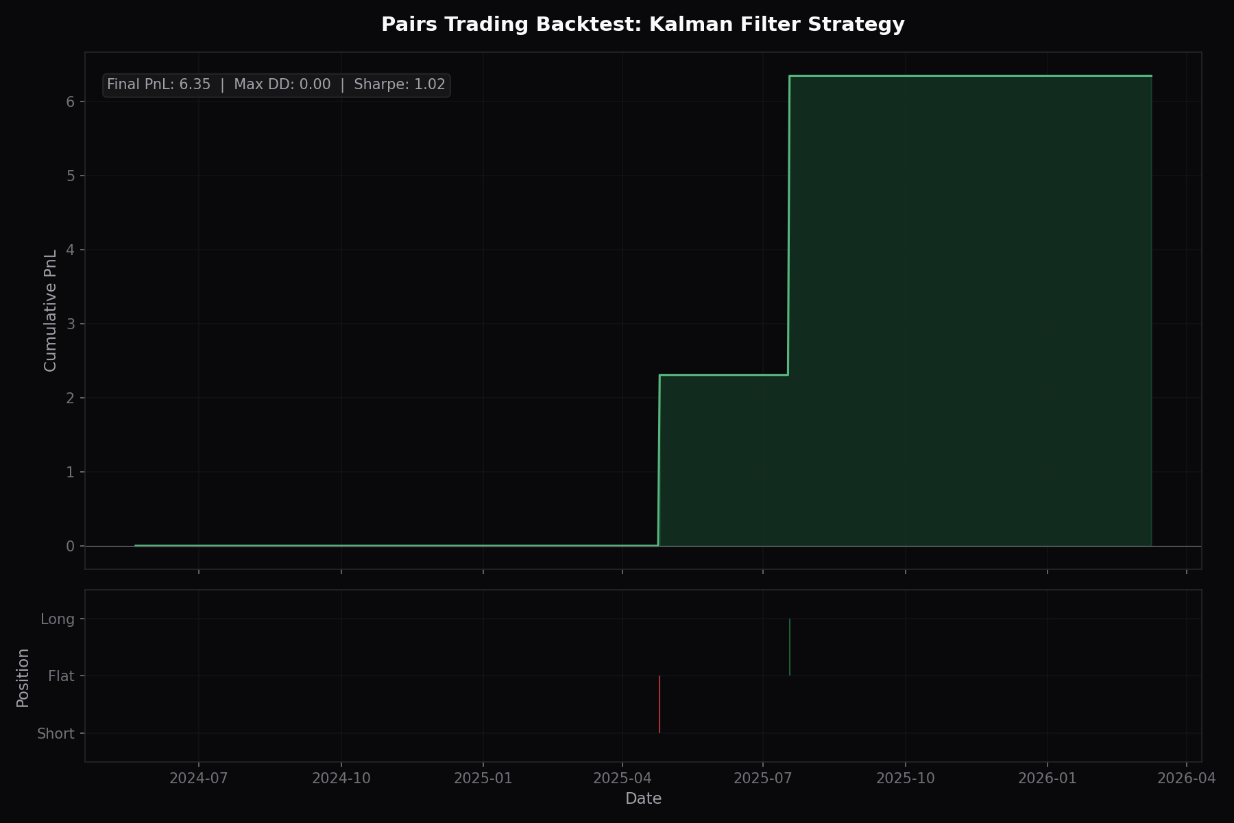
Equity curve from the backtest. The lower panel shows position: green is long spread, red is short spread. Notice how the strategy captures mean-reversion moves.
Tuning the Filter Parameters
The Kalman filter has two key parameters that control its behavior, and getting them right matters more than you might think.
δ (delta) - State Transition Variance
This controls how much α and β are allowed to change each period. Think of it as the filter's "memory."
High δ (e.g., 1e-3): The filter adapts quickly to new data. Good when relationships change fast. Bad because it becomes noisy and generates false signals.
Low δ (e.g., 1e-5): The filter is very smooth and stable. Good for steady relationships. Bad because it's slow to adapt when the relationship genuinely changes.
Ve (Ve) - Observation Noise Variance
This represents how much noise is in your price observations. It determines how much the filter trusts new data versus its internal model.
High Ve (e.g., 1e-2): The filter discounts observations heavily. Estimates are smooth but potentially lagged.
Low Ve (e.g., 1e-4): The filter reacts strongly to every observation. Fast adaptation but can overfit to noise.
How to tune them?
Start with δ=10−4 and Ve=10−3 as baselines. Then:
Run walk-forward optimization: Train on 1 year, test on 3 months, roll forward.
Check that performance is stable across different parameter values. If tiny changes blow up your Sharpe, you're overfitting.
Look at the hedge ratio plot. If it's jittering wildly, increase δ or decrease Ve. If it's not responding to obvious regime changes, do the opposite.
Sanity check: The z-score should have roughly unit variance. If it's consistently 3+ or 0.3, your parameters are off.
Extending the Framework
Once you have the basic Kalman pairs filter working, there are several directions to explore:
Multiple pairs: Run independent filters on multiple pairs. Diversification reduces single-pair blowup risk. Target uncorrelated pairs - don't just trade KO/PEP, KO/DPS, and PEP/DPS together.
Dynamic position sizing: Size positions inversely to spread volatility. When St is high, the spread is volatile and you should trade smaller. When it's low, you can be more aggressive.
Cointegration testing: Use the Kalman filter residuals to test whether the pair is still cointegrated. If the Augmented Dickey-Fuller test on recent spreads stops rejecting the unit root null, the pair may be breaking down.
Regime detection: Add a regime-switching layer. In high-volatility regimes, widen your entry thresholds or reduce position sizes. The Kalman filter can be combined with Hidden Markov Models for this.
Higher-frequency trading: Everything we've discussed works on intraday data too. The math is the same; the parameters are different.
Key Takeaways
Let me leave you with the core insights:
Static hedge ratios decay. If you're running pairs with OLS regression from 6 months ago, you're trading on stale information.
The Kalman filter makes your hedge ratio adaptive. It balances model predictions against new observations, updating estimates in real-time.
The innovation is your spread. The prediction error from the Kalman filter has known statistical properties, making z-score thresholds meaningful.
Parameter tuning matters.δ and Ve control the filter's responsiveness. Get them wrong and you'll either chase noise or miss real signals.
Pairs trading still has risks. Structural breaks, liquidity crises, and crowded trades can all blow you up. The Kalman filter helps but doesn't eliminate these risks.
The real edge isn't in knowing about Kalman filters - that's table stakes now. The edge is in rigorous implementation, disciplined risk management, and continuous research to stay ahead of the competition.
End of entry
Found this useful?
Likes decide what gets written next.Sign in to like
QuantFrame
Liked this article?
QuantFrame teaches you the math, code, and projects to break into quant. Plus a personalized roadmap built for your background and goals.