Five Free Interactive Sites That Teach the Maths Behind Quant Finance

Five websites, all free, no sign-up. Each one takes a piece of maths that quant work runs on and lets you move it with your mouse: probability, PCA, gradient descent, Markov chain Monte Carlo and Gaussian processes.

For each one: what it covers, the one experiment worth running on it, and where it shows up in quant work. I reran two of those experiments on real data. At the end: the one thing all five sites leave out, and twenty lines of numpy that fill the gap.

Seeing Theory Makes the Central Limit Theorem Earn Its Bell Curve

Built at Brown by Daniel Kunin, Jingru Guo, Tyler Dae Devlin and Daniel Xiang: six chapters from basic probability to regression, and every section has something to click.

Open the central limit theorem section in chapter 3. Shape the population with the two Beta sliders until it is lopsided, set the draws high, keep the sample size at 1 and press Sample: the sample means just copy the lopsided population. Raise the sample size and the bell appears. You are watching

$\bar{X}_n \approx \mathcal{N}\left(\mu, \frac{\sigma^2}{n}\right)$

become true, more slowly the more skewed the population. Every confidence interval on a strategy's average return leans on it.

Then do Prior to Posterior in chapter 5: set a Beta prior on a coin's bias, press Flip 10 times and watch the posterior narrow. For interviews, chapters 2 and 5, conditional probability and Bayes, are the ones to live in.

Open it: Seeing Theory

Setosa Shows How One Point Can Take Over the First Component

Victor Powell made the visuals and Lewis Lehe wrote the words. Drag any point in the height-and-weight example and the principal components, the directions the data varies most along, swing to follow. Then it takes a 3D cloud down to 2D and finishes on a real 17-variable table of UK diets, where Northern Ireland walks away from the other three countries.

Drag one point far out of the cloud and the first component turns toward it. PCA ranks directions by variance, variance squares distances, so one distant point gets a loud vote. In a matrix of returns, that point is a crash day.

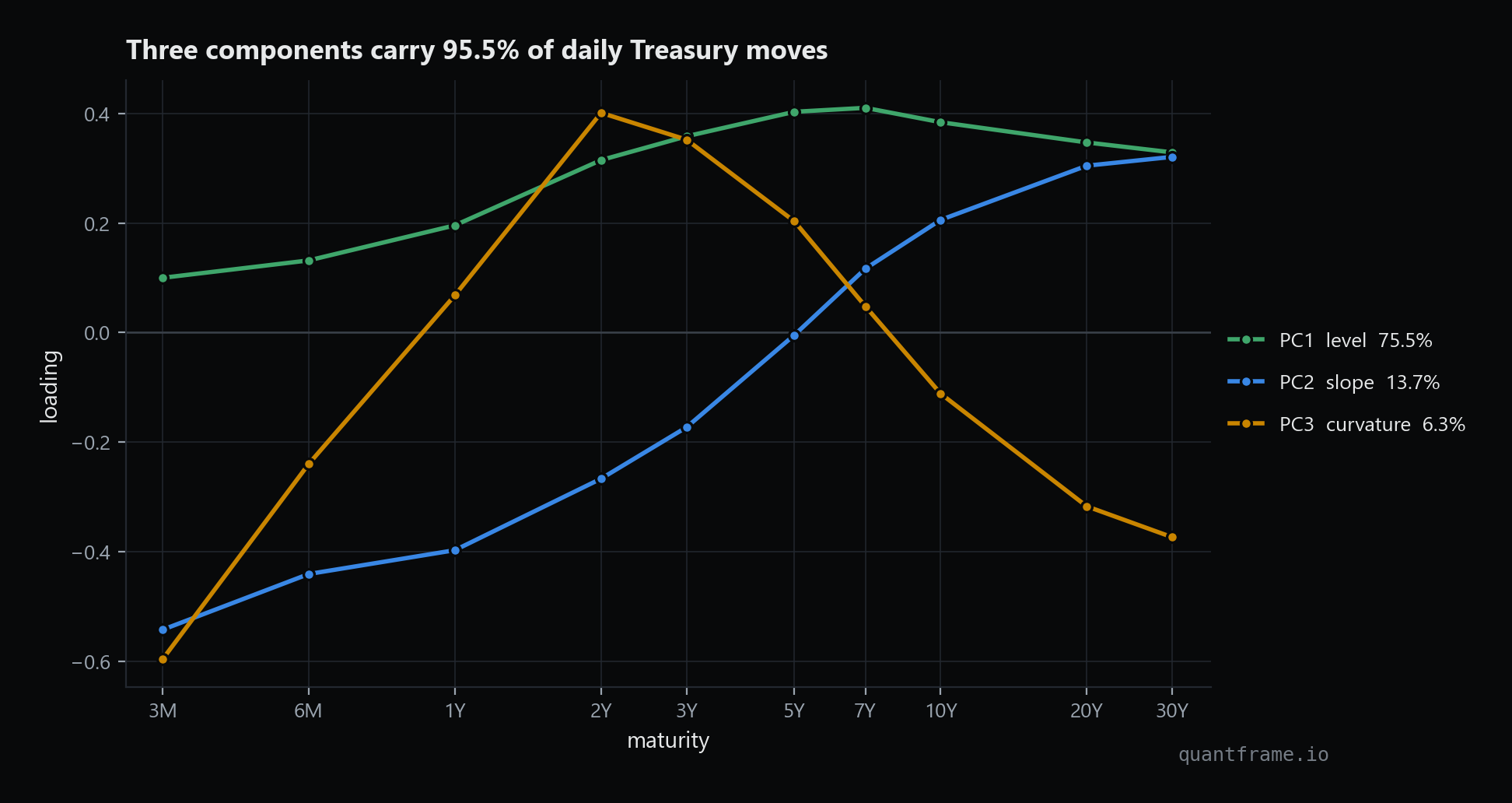
Then point it at real data. I ran PCA on 5,154 daily moves in US Treasury yields, ten maturities from 3 months to 30 years, February 2006 to September 2026.

Three shapes carry 95.5% of the variance: every maturity moving together (75.5%), the curve tilting (13.7%), and the middle bending against both ends (6.3%). Robert Litterman and José Scheinkman named them level, steepness and curvature in 1991 and pitched them as a hedging tool. The algorithm found all three with no idea what a bond is.

Open it: Principal Component Analysis Explained Visually

Distill's Momentum Article Turns Step Sizes Into Arithmetic

Gabriel Goh's 2017 article rewrites gradient descent on a quadratic bowl in the eigenvectors of its curvature matrix, where every direction converges on its own and at its own speed. The sliders for step size and momentum sit right beside the maths.

Push momentum toward 1 in the first figure and the path starts to swing; push the step size and it leaves the plot. The article then shows why. Speed is set by the condition number $\kappa$, the largest curvature divided by the smallest, and with the best settings each step shrinks the error by a factor of

$\text{gradient descent: } \frac{\kappa-1}{\kappa+1} \qquad \text{momentum: } \frac{\sqrt{\kappa}-1}{\sqrt{\kappa}+1}$

The covariance matrix behind the Treasury figure is the curvature of any risk-minimisation problem across those ten maturities, and its condition number is 465. With Goh's optimal settings, gradient descent took 2,973 iterations to cut the error a millionfold. Momentum took 200. Fifteen times fewer steps, read straight off one number.

Open it: Why Momentum Really Works

The MCMC Gallery Makes Picking a Sampler a Decision

Markov chain Monte Carlo draws samples from a distribution you can only evaluate up to a constant, which is where every Bayesian model leaves you. Chi Feng's gallery has 13 samplers, from random-walk Metropolis-Hastings through Hamiltonian Monte Carlo (HMC), NUTS, Gibbs and the Langevin-based MALA, one click each, all opening on the same banana-shaped target.

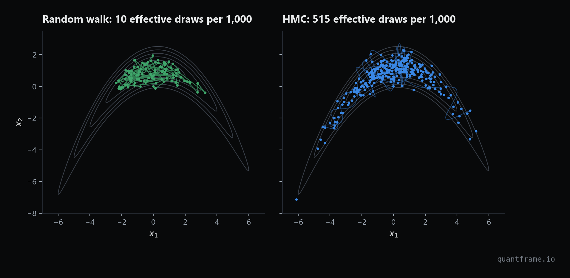
Run the random walk on the banana, then HMC. I rebuilt both with the gallery's own target and default settings:

An effective draw is what a correlated chain is worth in independent samples. Per step, HMC gets over 50 times more of them. Per unit of compute, counting its 37 gradients a step, the gap on this 2D toy shrinks to 1.4 times. Radford Neal's scaling analysis puts the random walk's cost at $d^2$ in $d$ dimensions against $d^{5/4}$ for HMC, so at a few hundred parameters the choice makes itself. Stan and PyMC both default to NUTS, the self-tuning HMC in the gallery.

Open it: The Markov-chain Monte Carlo Interactive Gallery

The Gaussian Process Article Shows Where a Model Stops Knowing

Jochen Görtler, Rebecca Kehlbeck and Oliver Deussen build Gaussian processes, probability distributions over whole functions, up from the multivariate normal, through kernels (the rule for how strongly two points move together) to prior and posterior. Every figure moves.

In the posterior figure, click the training points on one at a time: the uncertainty band pinches shut around each one and stays wide in the gaps. In the last figure, fit the rising, wavy data with the RBF kernel alone and watch the prediction drift back to the prior mean once it leaves the data. Add linear plus periodic and it keeps the trend.

That drift is the honest part. A GP tells you where it is interpolating and where it is guessing, the question to ask of any curve drawn through sparse quotes. It leans on everything above it, which is why it goes last.

Open it: A Visual Exploration of Gaussian Processes

You Understand a Sampler Once You Have Written One

All five sites share one limit: you are watching. A slider shows you what happens but never makes you decide anything, and deciding is where the understanding comes from. What step size? Where does the chain start? How many draws are worth keeping?

So write one. Here is the gallery's random walk on the gallery's banana, in about twenty lines of numpy:

import numpy as np

MU = np.array([0.0, 4.0])
S_INV = np.linalg.inv([[1.0, 0.5], [0.5, 1.0]])


def log_banana(x, a=2.0, b=0.2):
    """The gallery's banana: a correlated Gaussian bent by a quadratic."""
    y = np.array([x[0] / a, a * x[1] + a * b * (x[0] ** 2 + a ** 2)])
    d = y - MU
    return -0.5 * d @ S_INV @ d


def random_walk_metropolis(log_p, x0, n_steps=5_000, step=1.0, seed=0):
    rng = np.random.default_rng(seed)
    x = np.asarray(x0, dtype=float)
    lp, chain, accepted = log_p(x), [x], 0
    for _ in range(n_steps):
        proposal = x + step * rng.standard_normal(x.size)  # propose
        lp_new = log_p(proposal)
        if np.log(rng.uniform()) < lp_new - lp:  # accept...
            x, lp, accepted = proposal, lp_new, accepted + 1
        chain.append(x)  # ...or count the old point again
    return np.array(chain), accepted / n_steps


chain, rate = random_walk_metropolis(log_banana, x0=[0.0, 0.0])
print(f"accepted {rate:.0%} of proposals")

It accepts 36% of its proposals. Set step to 0.1, then to 3, and plot the chain each time. Somewhere between those two runs the animation turns into something you could explain to someone else.

That loop, watch it and then build it, is how QuantFrame is put together. Four of these five sites have a QuantFrame module behind them (probability, linear algebra with PCA, optimisation, computational methods), and in the Metropolis-Hastings lesson you run the sampler in your browser on a Bayesian model of an asset's drift and check it against the exact answer.

The sites give you the picture. When you want to build what is behind it, your roadmap is waiting at quantframe.io.