21.6 million real poker hands. Two million zeros of the Riemann zeta function. 727 million rows of Polymarket against Binance. Three years of Ethereum's public mempool, archived daily.
All four are free, and a useful slice of each downloads in minutes.
A dataset on your drive proves nothing; what you compute from it is the project. So I pulled a real slice of each one, ran the first measurement a serious project would start from, and worked out what is worth building on top. Each section ends with its link. At the end: which one to pick for the job you want.
21.6 Million Poker Hands Are a Skill-Versus-Luck Lab
The University of Toronto's Computer Poker Research Group converted 21,605,687 real no-limit hold'em hands into one open format: anonymised logs from six online sites over 23 days in July 2009, stakes 25NL to 1000NL. The repo also carries all 10,000 hands Pluribus played against professionals, every hole card shown.
Each hand is a few lines of TOML: blinds, stacks, every action in order. The pokerkit library replays them.
python
from pokerkit import HandHistory

with open("phh_abs600/abs_NLH_handhq_1-OBFUSCATED.phhs", "rb") as f:
    hands = list(HandHistory.load_all(f))

for hh in hands[:3]:
    for state in hh:  # replays the hand, action by action
        pass
    print(hh.actions[-2:], [float(x) for x in state.payoffs])
Two facts decide what you can build. Hole cards appear only at showdown; everything else is ????. And the stored winnings field is unreliable, so take payoffs from the replay (they are before rake).
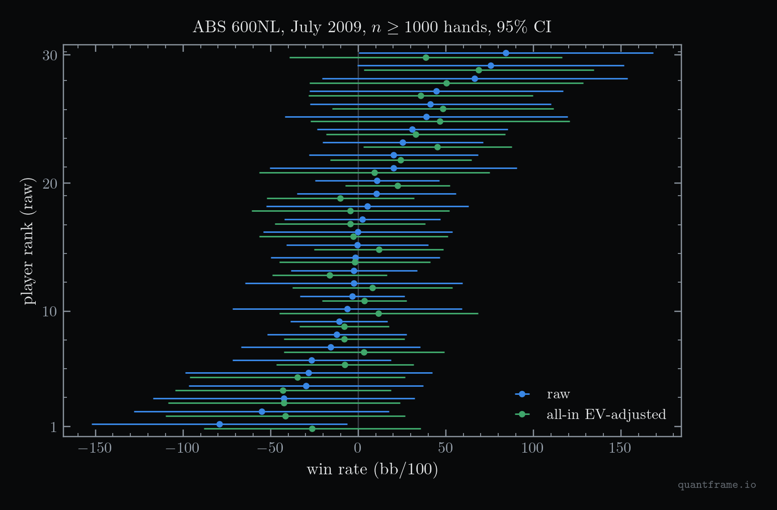
I took one complete folder, Absolute Poker 600NL, 6-max: 40 files, 39,282 hands, 777 players. The median player has 69 hands; thirty have more than 1,000. Which of those 30 are good?
The 30 regulars with 1,000+ hands. Two clear zero on raw results; strip out all-in luck and two different players do. Thirty coin-flip players would produce 1.5 on average.
Per hand, a regular's result has a standard deviation of 11.4 big blinds. A genuine winner at 5 big blinds per 100 hands needs about 201,000 hands before a 95% interval clears zero. The best-sampled player in the folder has 4,678.
Project 1: run the fund-manager skill test on poker players. First cut variance: when two players are all in with both hands shown, only the remaining cards decide the result, so replace it with its expectation:
lucki=payoffi−(equityi⋅pot−contributioni)
Here, 831 heads-up all-ins, 2.1% of hands, carry 20.3% of all payoff variance. Then apply the false discovery rate method Barras, Scaillet and Wermers built for mutual fund alpha to estimate the share of truly skilled players, and test persistence: rank on July 1 to 11, check on July 12 to 23. Potter van Loon, van den Assem and van Dolder put the point where skill outweighs luck at about 1,500 hands; test that with luck removed.
Project 2: measure tilt with a natural experiment. Who wins an all-in runout is pure chance, so the luck term is a randomised treatment. Regress a player's next 50 hands on it: hands played, raise frequency, bet sizes, leaving the table, moving stakes. Smith, Levere and Kurtzman found players play less cautiously after big losses, and Eil and Lien found a break-even effect in 9.1 million Full Tilt hands, both with results that mix skill and luck. It is the question Coval and Shumway asked of Chicago bond futures traders who took more risk in the afternoon after losing in the morning.
Project 3: price river bets like a market maker. A river bet is an order; the caller is the dealer deciding whether to trade against it. The replay names the winner of every called river bet even when the loser mucks, so the caller's average result by bet-to-pot ratio is a markout curve. The benchmark: against a bet of b into a pot of P, a balanced bettor bluffs b/(P+2b) of the time. Pluribus's hands are the near-equilibrium reference, and the population's distance from it is an edge in big blinds.
Open it:uoftcprg/phh-dataset on GitHub. The full zip is 1.9 GB; one stake folder is a sparse checkout. Skip iPoker for anything involving money: its stacks are recorded as infinite.
The Zeros of the Zeta Function Behave Like a Random Matrix
Andrew Odlyzko spent decades computing zeros of the Riemann zeta function and left the results on his University of Minnesota page as plain text, one number per line. The first file holds the first 100,000 zeros to within 3×10⁻⁹, in 1.8 MB. Another holds the first 2,001,052. Three more hold 10,000 zeros each from far up the critical line, just past zero number 1012, 1021 and 1022; the last opens at height 1,370,919,909,931,995,308,226.68.
Each line is the γn of a zero at 21+iγn, and the gaps are the story. In 1972 Hugh Montgomery was at afternoon tea in Princeton with a formula for how pairs of zeros are spaced, and Freeman Dyson recognised it on the spot as the pair correlation of eigenvalues of large random Hermitian matrices:
R2(u)=1−(πusinπu)2
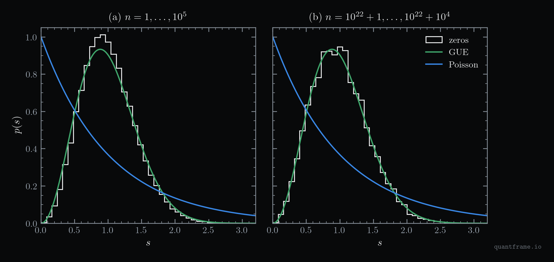
Rescale the zeros so the average gap is 1 (the Riemann-Siegel theta function does it exactly) and the test takes a minute:
Gaps between consecutive zeros against the Gaussian Unitary Ensemble and against independent random points. Near zero 10²² the zeros sit on the random-matrix curve; the first 100,000 overshoot its peak, a finite-height correction.
The zeros repel each other. Independent points would put 9.5% of gaps below 0.1; near zero 1022 it is 0.07%. The gap variance there is 0.176, against 0.180 for the random-matrix ensemble and 1 for independent points, drifting up from 0.161 for the first 100,000 zeros. Nothing is fitted.
Project 1: calibrate a random matrix toolkit on the primes, then point it at the market. The same mathematics cleans covariance matrices: Laloux, Cizeau, Bouchaud and Potters found 94% of the eigenvalues of a 406-stock correlation matrix inside the band pure noise would produce, and Plerou and coauthors found stock eigenvalue spacings repel with exponent 0.99 ± 0.02, against 2 for the zeros. Build the tools (unfolding, spacing distributions, number variance, a Brody fit) and validate them on the zeros, where the answer is known. Then clean a stock covariance with Marchenko-Pastur clipping and Ledoit-Wolf shrinkage and backtest out-of-sample minimum-variance portfolios. The benchmark: in Plerou's 2002 study the raw matrix underestimated next year's realised portfolio risk by about 170%, the filtered one by about 25%.
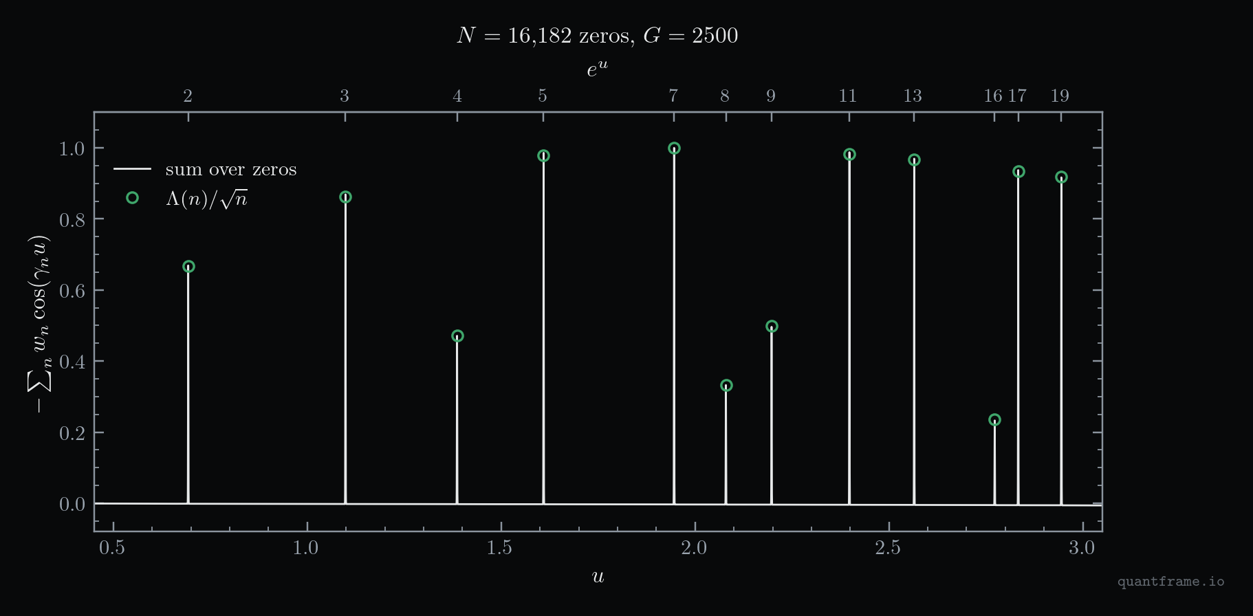
Project 2: hear the primes. The explicit formula ties the zeros to the primes. Add the zeros up as cosine waves with a Gaussian taper,
F(u)=−∑nwncos(γnu),wn=e−γn2/2G2,
and every prime power n=pk produces a spike at u=logn with height proportional to Λ(n)/n, where the von Mangoldt function Λ(n) equals logp.
16,182 zeros, taper G = 2500. Every prime power below 20 appears, and the open circles are the predicted heights, matched to 0.5%. The zeros know where the primes are.
Then run it backwards: rebuild the prime-counting staircase ψ(x) from the zeros and watch it sharpen as you add more. You meet the problem every spectral analysis of returns has: truncate a sum of waves without a taper and it rings until the signal drowns. Stretch goal: scan all two million zeros for Lehmer pairs, neighbours that almost collide, the objects that pushed lower bounds on the de Bruijn-Newman constant up toward zero before Rodgers and Tao proved it is at least 0.
Open it:Odlyzko's zeta tables. Unfold the high zeros from the file's offsets: float64 cannot hold a base near 1021 plus an offset.
OpenMarket Puts Polymarket and Binance on One Millisecond Clock
Polymarket runs a market every 15 minutes on one question: will Bitcoin finish the window at or above where it started, as measured by Chainlink's BTC/USD data stream? In July, Gregory Young at CU Boulder released OpenMarket: 727,098,247 rows covering 4,450 of these markets from February to May 2026, Polymarket order book updates next to Binance BTC/USDT trades, timestamped to the millisecond.
The paper began as an attempt to trade these markets. A 43-feature model, retrained walk-forward, scored an AUC of 0.8377. The plain Polymarket mid scored 0.8405. With a 1% fee and 0.5% slippage the simulated strategy lost 0.116 normalised payoff units per attempted trade. The headline result is a null result, and the dataset is what survived.
That makes the market price the benchmark to beat, so I priced the contract from first principles. Up is a cash-or-nothing digital option struck at the open:
P(up)=Φ(στln(St/K))
K is the Chainlink opening price (the dataset has no outcomes; Polymarket's Gamma API does), St is Binance minus the opening basis (median 9.02 USD), σ the realised volatility of the previous 30 minutes and τ the seconds left. I ran it on all 92 complete markets of 4 April 2026, a Saturday.
python
def binance_at(t):
    i = np.searchsorted(bts, t, side="right") - 1
    return bpx[i]

basis = binance_at(m.t0) - m.K                        # Binance minus Chainlink at the open
hist = binance_at(np.arange(m.t0 - 1_800_000, m.t0 + 1, 1000))
sig = np.sqrt(np.mean(np.diff(np.log(hist)) ** 2))    # per sqrt(second), last 30 minutes
S = binance_at(grid) - basis
tau = (m.t0 + 900_000 - grid) / 1000                  # seconds to expiry
p_up = norm.cdf(np.log(S / m.K) / (sig * np.sqrt(tau)))
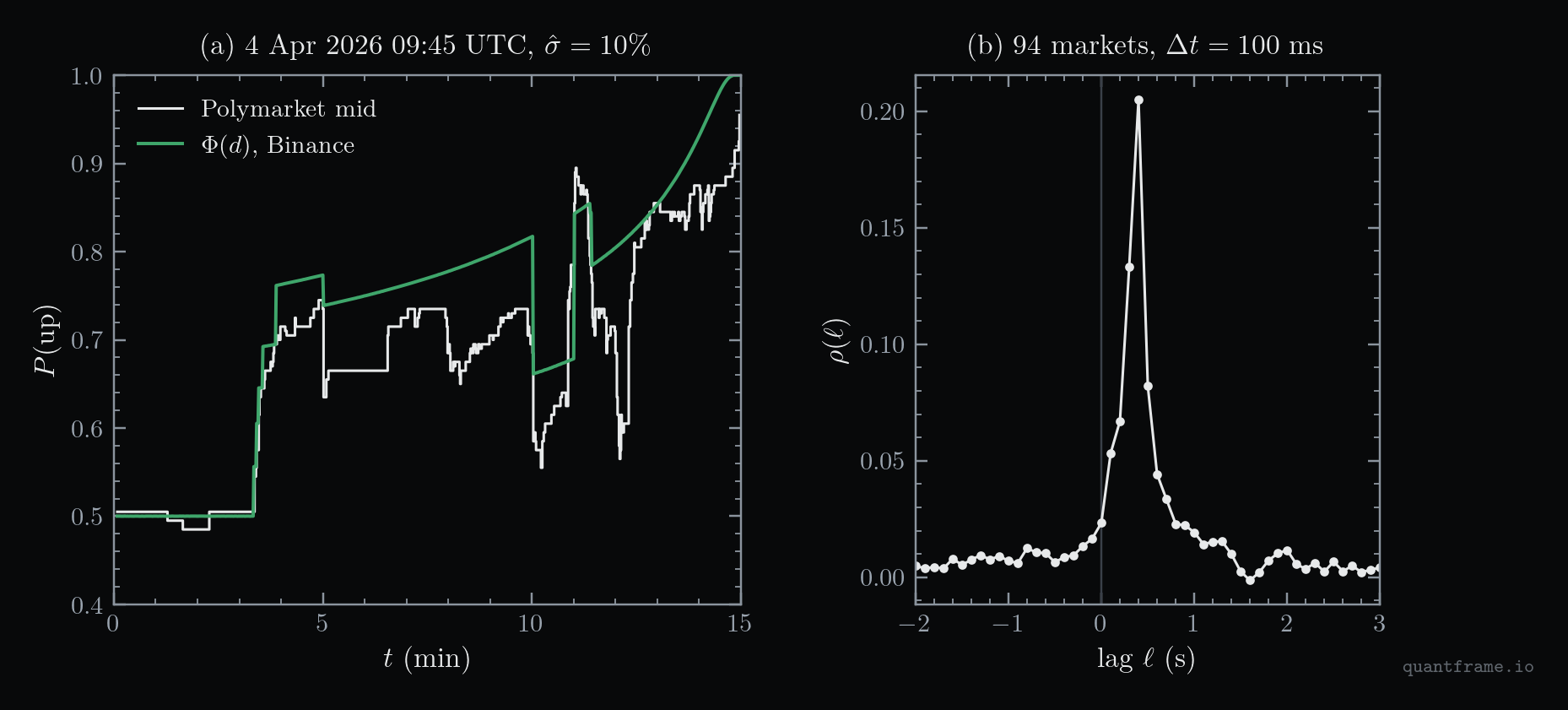
(a) One window, 09:45 UTC. From minute 5.5 to 10 Binance moved one cent, the formula climbed toward 1 as time ran out, and the market sat up to 0.13 below it. (b) Cross-correlation of 100 ms moves over 94 markets: Polymarket follows Binance, peaking 0.4 seconds later.
Across all 92 markets formula and market correlate at 0.95, yet the formula lands inside the bid-ask quote only 1 to 5% of the time. Five to ten minutes out it matches the market on Brier score (0.174 against 0.177). In the last 30 seconds it collapses: 0.196 against 0.121. The prime suspect is the basis: settlement is on Chainlink, and the Binance-Chainlink gap moved with a standard deviation of 5.41 USD within a window, a lot when the price sits a few dollars from the strike.
Project 1: build the implied volatility surface of a 15-minute binary. Invert the mid for σ every second and map the result against time to expiry and distance to strike. Then fix the model where it breaks: give the basis its own noisy process, add jumps, and score each version by Brier against real Chainlink outcomes. The goal is a model that beats the mid in the final minutes after the taker fee, 0.07⋅p(1−p) per share since 30 March 2026, or 1.75 USDC per 100 shares at a price of 0.5.
Project 2: measure price discovery properly. The 0.4-second peak is the crude version; the paper's clock-free event study puts the median response at 347 ms. Use the Hayashi-Yoshida estimator on raw asynchronous ticks, turn the Polymarket mid into an implied Bitcoin price through the inverse digital so both series are in dollars, and compute information shares. Then backtest the obvious latency trade with the real fee curve and spread. Expect it to fail, and report exactly where the edge dies.
Project 3: simulate a market maker and score it with Binance markouts. Every Polymarket price-level change is in the data, so you can rebuild the book and post simulated quotes. Makers pay no fee and get 20% of taker fees back; the cost is adverse selection, measured as how far Binance moves 1, 5 and 30 seconds after each fill. There are no trade prints or queue positions, so count a fill only when the opposite quote moves through your level.
Before a transaction lands in an Ethereum block it usually waits in the mempool, the public waiting room every node can see. Flashbots has archived it daily since August 2023: every unique transaction, the millisecond it was first seen, its fees, the full signed payload, and whether and when it landed on-chain. Daily Parquet files, public domain, also on BigQuery and Dune.
One day, 27 September 2026 (a Sunday), is a 230 MB file of 788,790 transactions from 216,930 senders. 97.9% were included. The median transaction landed 6.0 seconds after it was first seen, the 99th percentile after 62 seconds.
What the file does not contain is the interesting part. An on-chain transaction missing from the archive never passed through the public mempool. It reached a block builder privately, through a protected RPC, an order flow auction or a searcher's bundle.
python
import pyarrow.parquet as pq
import requests

# https://mempool-dumpster.flashbots.net/ethereum/mainnet/2026-09/2026-09-27.parquet (230 MB)
hashes = pq.read_table("mempool_2026-09-27.parquet", columns=["hash"]).column("hash")
public = {h.lower() for h in hashes.to_pylist()}

body = {"jsonrpc": "2.0", "id": 1, "method": "eth_getBlockByNumber",
        "params": [hex(26_068_000), True]}
block = requests.post("https://eth.drpc.org", json=body).json()["result"]
seen = [tx["hash"].lower() in public for tx in block["transactions"]]
print(f"{sum(seen)} of {len(seen)} transactions were ever public")
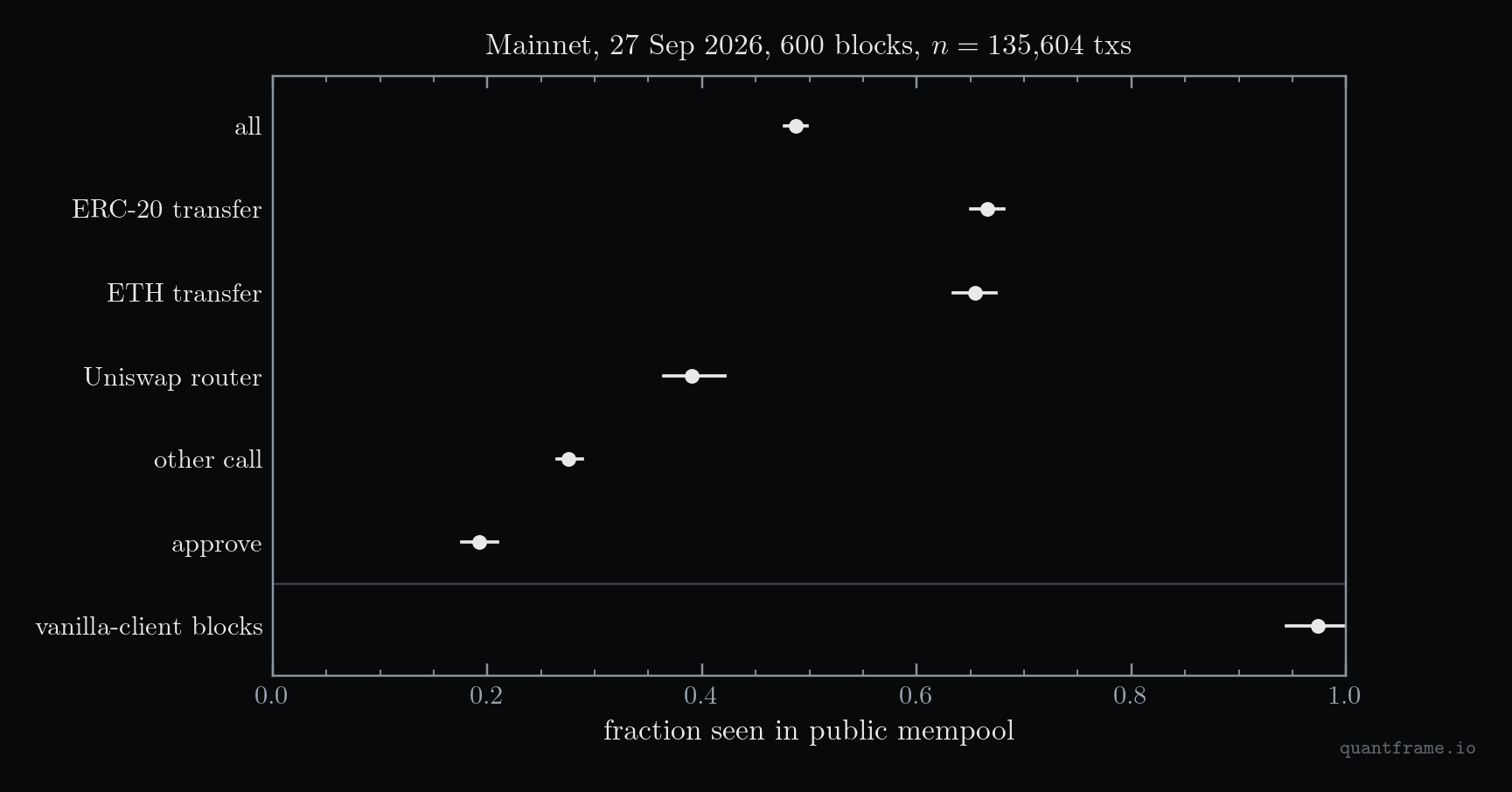
I ran that join on 600 random blocks from the same day, 135,604 transactions.
Share of on-chain transactions ever seen in the public mempool, 95% block-bootstrap intervals. The bottom row is the control: blocks built by an ordinary client fill from the public mempool, and the archive catches 97% of their transactions.
48.7% of on-chain transactions were ever public (95% interval 47.7 to 49.8). Transfers are mostly public, about two thirds. Uniswap router swaps 39%, token approvals 19%. The first transaction in a block, where builders and bots put their own trades, was public 12.6% of the time.
Project 1: build the private order flow meter, 2023 to 2026. Wang and coauthors, on the same archive for November 2023 to May 2024, found private transactions were 12% of transactions but 54.59% of block rewards. Mancino and Rezzoli measured 31.8% private in November 2024 and 50.1% by February 2025; this Sunday says 51%. Run the join for every day, split it by builder and contract, and keep the ordinary-client blocks as a coverage check: Heimbach and coauthors warn that archive outages misclassify public transactions as private, which is exactly what the control row catches.
Project 2: build a sandwich calculator from the victim's own settings. A public swap broadcasts its slippage tolerance. Decode Uniswap V2 router swaps from the raw transaction (amount in, minimum out, token path), rebuild the pool's reserves at the previous block, and the maximum sandwich profit follows in closed form from x⋅y=k. Validate against Dune's labelled sandwiches and you get the price of a loose slippage setting by trade size, and how much of it was taken. Mancino and Rezzoli found about 40% of sandwich victims switch to private routing within 60 days; your calculator shows what they paid before they did.
Project 3: model time to inclusion like a limit order's time to fill. A pending transaction is a limit order in a priority auction: the tip is its price, inclusion its fill. That day, transactions tipping 0.001 gwei or less had a 90th-percentile wait of 43 seconds; at 1 to 2 gwei, 9.8 seconds. Fit a discrete-time hazard model per block on tip relative to base fee, gas and hour, treat never-included transactions as censored and replacements (same sender and nonce resubmitted, 3,908 cases that day) as a competing risk. It is the fill-probability model from limit order books.
Open it:mempool-dumpster.flashbots.net. One trap: the per-source columns, which recorded which data provider saw each transaction first, have been empty since 15 July 2025.
What This Means For You
1. Pick the dataset by the job you want. Poker is skill measurement and behavioural finance, a quant researcher's language. The zeta zeros are random matrix theory, the toolkit behind covariance cleaning. OpenMarket is pricing, price discovery and market making, desk work. The mempool is market microstructure with the order flow in the open.
2. A clean negative result counts. OpenMarket's paper is a null result and still useful. A latency strategy that dies after fees, with the autopsy written up, tells an interviewer more about you than a Sharpe ratio of 4.
3. Read each dataset's blind spots first. Hole cards only at showdown. No outcomes in OpenMarket. Empty source columns in the mempool archive since July 2025. Each quietly ruins a project if you find it after the analysis.
Every project here sits on the same foundations: probability, linear algebra, statistical computing, and Python that can chew through a few hundred million rows. QuantFrame teaches exactly those, with interactive problems and projects where you build it yourself. Your personalized roadmap is at quantframe.io.
End of entry
Found this useful?
Likes decide what gets written next.Sign in to like
QuantFrame
Liked this article?
QuantFrame teaches you the math, code, and projects to break into quant. Plus a personalized roadmap built for your background and goals.