Five Repos, One Engine: Wiring the Open-Source Quant Stack

J.P. Morgan built a trading grid, ran it on their own trader desktops, then gave it away. The FINOS case study that documents the open-sourcing puts it "in production use in 1,000's of applications within J.P. Morgan including trader desktops". RBC Capital Markets took the free version, piloted it, and rolled it out to 300+ users on their own trading floor.

That grid is called Perspective. It is one of five open-source repos that, between them, cover the jobs a systematic trading operation actually pays for: pricing, risk, portfolio construction, execution, display.

Here is the part that bothered me enough to write this. None of the five knows the others exist. There is no tutorial, no glue repo, no blog post wiring them into one system. Five engines, zero drivetrain.

So I built the drivetrain. Everything below ran on my laptop this week, in one Python 3.13 environment, on Windows, starting from a single line:

bash

pip install perspective-python QuantLib open-source-risk-engine skfolio nautilus_trader

All five import into one process. The versions in this article: Perspective 5.3.0, QuantLib 1.43, ORE 1.8.16.0, skfolio 1.0.2, NautilusTrader 1.231.0. Every number below was computed in that environment, and where something broke, I will show you exactly where, because the breakage is the part no listicle will ever tell you about.

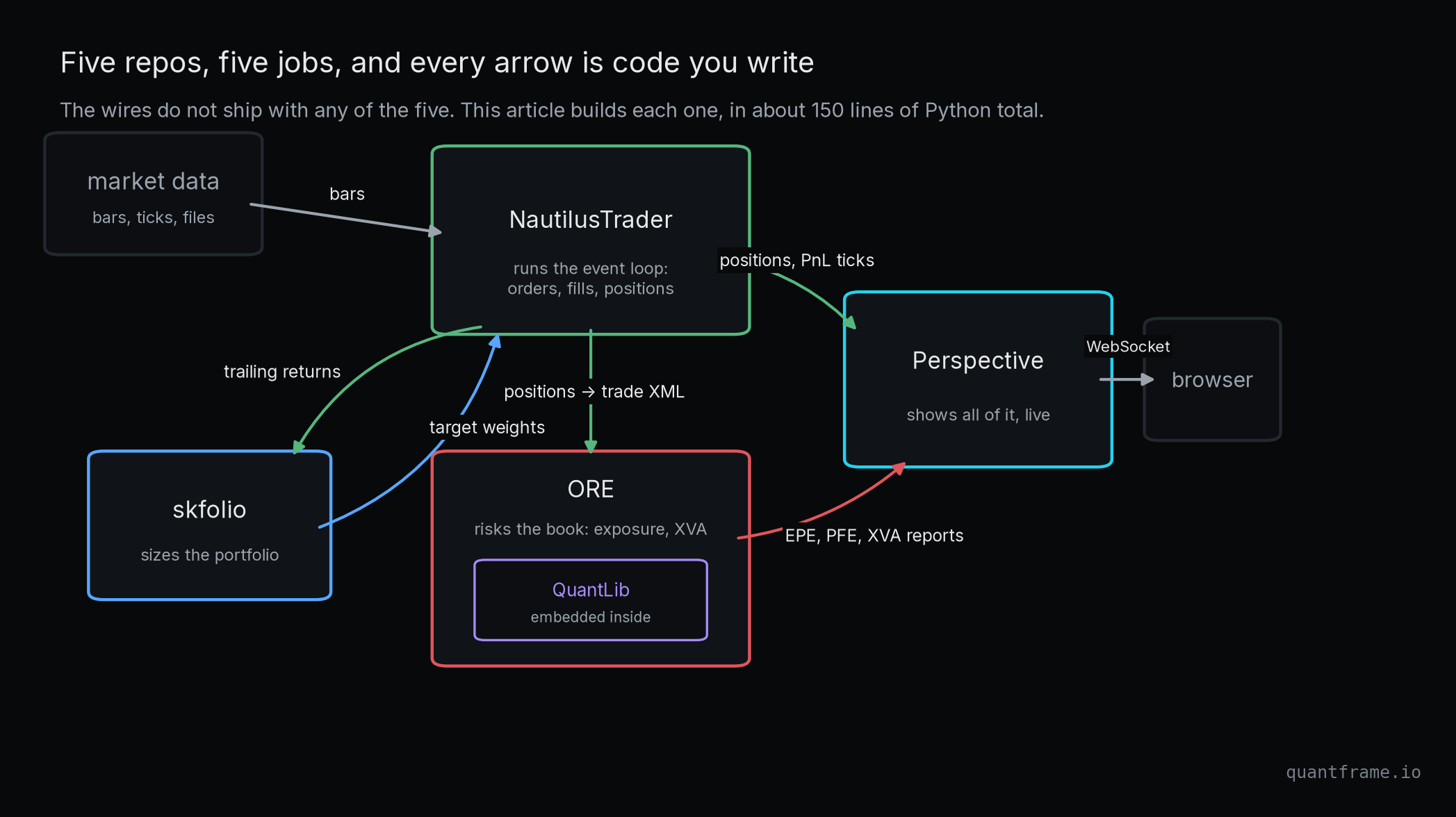
Architecture diagram of the five-repo quant stack: NautilusTrader at the center, skfolio, ORE with QuantLib embedded, Perspective and the browser, with labeled data contracts on every arrow — The engine, assembled. Every box ships for free; every arrow is your job.

The Stack Is Five Jobs, and the Wires Are Missing

Strip a quant operation down and five jobs remain.

Something prices instruments: QuantLib, 7,555 stars, shipping since 2000, 18,879 commits deep. Something measures what the book can lose: ORE, built on top of QuantLib by people who sell risk systems to banks. Something decides position sizes: skfolio, portfolio optimization on the scikit-learn contract. Something turns targets into orders without leaking money: NautilusTrader, a Rust-core event engine with a Python API. And something puts live numbers in front of a human: Perspective.

The wires between them are data contracts, and there are only four you need to internalize. Returns flow into the allocator. Weights flow out of it. Orders and fills live inside the execution engine. Positions flow out to risk and to the screen.

Hold those four contracts in your head and the rest of this article is just filling in syntax.

QuantLib Is the Math Everyone Else Borrowed

QuantLib gets pitched as an option pricer. That undersells it in a specific way: the pricing models are the replaceable part. The irreplaceable part is the plumbing underneath: day count conventions, per-exchange holiday calendars, business day adjustment rules, schedule generation. Boring, unglamorous, and the actual reason a 20-year-old C++ library still ships a release every quarter like clockwork: v1.41 in January 2026, v1.42 in April, v1.43 in July.

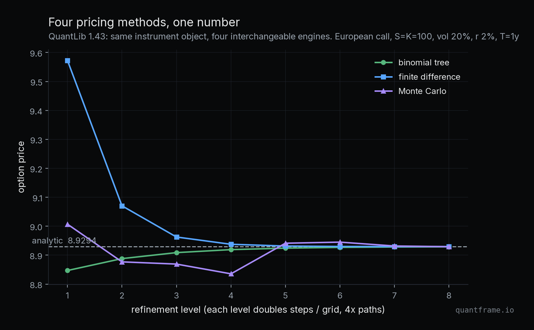
The architecture is one idea repeated everywhere: an instrument is an object, and pricing it is a separate, swappable engine. To see it, I priced one European call (spot 100, strike 100, vol 20 percent, rate 2 percent, one year) with four different engines: closed-form Black-Scholes, a binomial tree, finite differences, and Monte Carlo.

Convergence chart of binomial tree, finite difference and Monte Carlo option prices toward the analytic Black-Scholes value of 8.9294 as refinement increases — Analytic answer 8.9294. At full refinement the three numerical engines land within 0.0007 of it. The instrument object never changed.

Same instrument, four methods, one number: the tree ends at 8.9288, finite differences at 8.9295, Monte Carlo at 8.9292 against the analytic 8.9294. This matters for the stack because swaptions, callables and exotics have no closed form, and the engine you swap in is a one-line change.

One more thing I did not appreciate before this build. Install ORE and you get QuantLib twice: import ORE exposes the entire QuantLib API inside itself (ORE.Date, ORE.Settings, all of it) plus everything ORE adds on top. The QuantLib-to-ORE wire is the only one in the diagram you do not have to build. It ships pre-welded.

ORE Speaks XML, and the XML Is the Hard Part

ORE is what happens when a consultancy that builds risk engines for banks open-sources its core. Acadia (now part of LSEG Post Trade) sponsors it, and LSEG states plainly that ORE is "processing hundreds of thousands of trades per day in production services", with new models passing through LSEG's internal model risk governance before release. It has 779 GitHub stars. Bank quants do not star repos; judge it by the governance, not the glamour metrics.

What it computes is the risk layer of the stack: Monte Carlo simulation of your whole portfolio across future dates, exposure profiles per netting set (the legal grouping of trades that can be offset against one counterparty), and the XVA family on top. CVA alone, the credit valuation adjustment, is the market price of the risk that your counterparty defaults while owing you money:

$\mathrm{CVA} = (1 - R)\int_0^T \mathrm{EPE}(t)\, \mathrm{d}PD(t)$

where $R$ is the recovery rate, $\mathrm{EPE}(t)$ the discounted expected positive exposure at time $t$ , and $PD$ the counterparty's default probability curve.

You do not call ORE like a library. You describe everything in XML: the portfolio, the netting sets, the curve configurations, the simulation model, the pricing engines. Then Python is just the ignition:

run_ore.pypython

from ORE import Parameters, OREApp

params = Parameters()
params.fromFile("Input/ore.xml")   # points at portfolio, curves, simulation setup
ore = OREApp(params, True)
ore.run()

exposure = ore.getReport("exposure_nettingset_CPTY_A")
xva      = ore.getReport("xva")

Now the honest part. The shipped Python example does not run against the current pip wheel. I hit two failures and both are instructive. First, the example's pricing configuration asks for a swap engine (DiscountingSwapEngineOptimised) that exists in ORE's master branch but not in the 1.8.16.0 wheel; one name change in pricingengine.xml fixes it. Second, the market configuration lists the 6M discount curves but not the overnight curves they bootstrap against, and the wheel's dependency resolver will not find them on its own; three lines added to todaysmarket.xml fix that. Twenty minutes of reading ORE's structured error log, two small edits. That is the real cost of wiring bank-grade software, and it is worth paying because of what comes out the other side.

What came out: a 20-year euro interest rate swap, 10 million EUR notional, receiving 2 percent fixed against 6M Euribor, valued at 1,609,885.84 EUR. Then 1,000 Monte Carlo paths across 81 future dates, in 6.3 seconds, on a laptop.

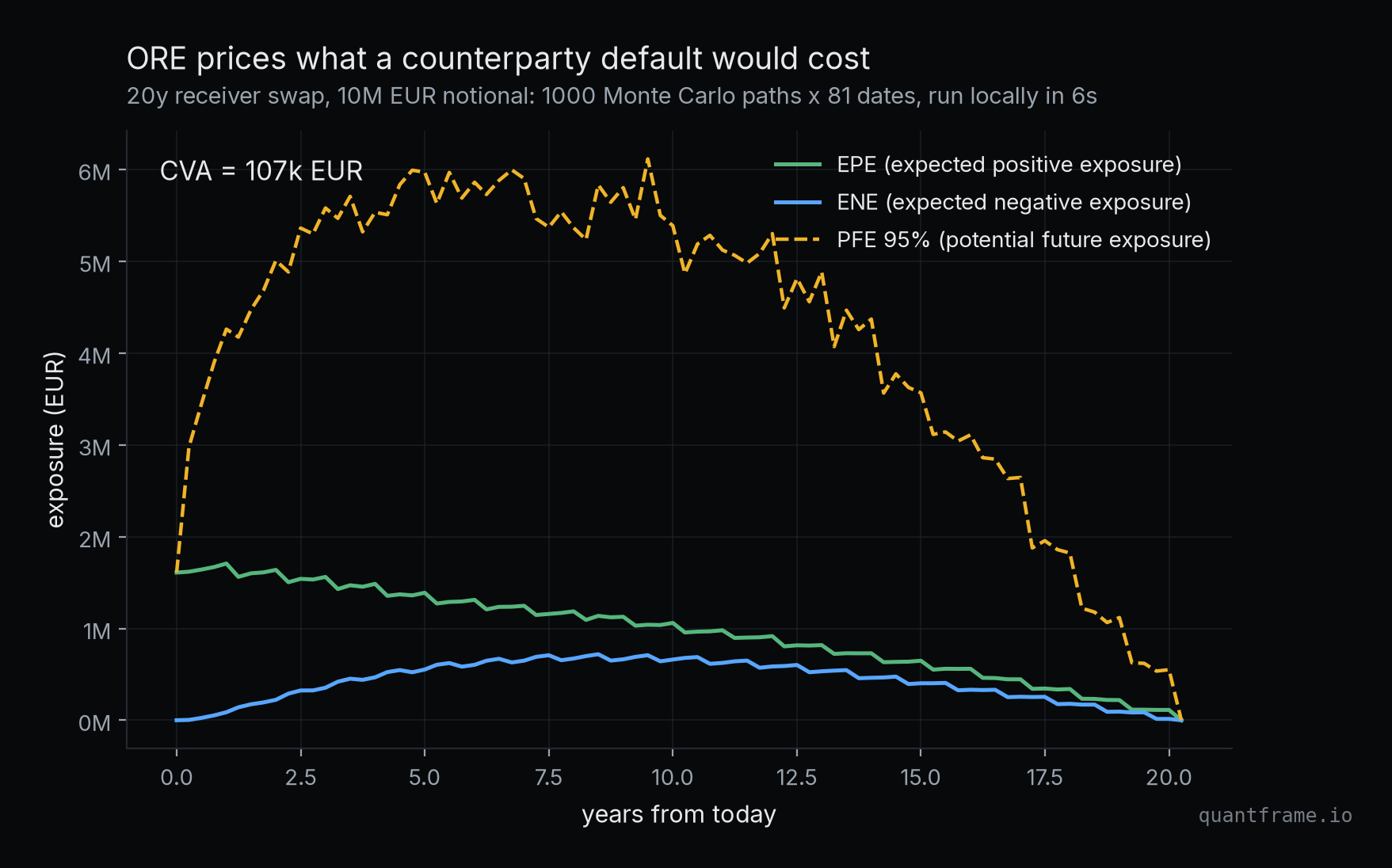
The lifetime of a swap's counterparty risk. Expected exposure peaks near 1.7M EUR while the 95th percentile touches 6.1M, and CVA prices the whole profile at 107k.

The exposure profile has the classic swap shape: it rises as rates get time to drift, peaks mid-life, then amortizes to zero as remaining cashflows run out. Expected positive exposure peaks around 1.71M EUR. The 95 percent potential future exposure, the number a credit officer would set limits against, touches 6.11M. And the CVA on the netting set comes out at 107,446.98 EUR, about 1 percent of notional, which is the amount a desk would need to be paid to carry this counterparty's default risk unhedged.

This is the calculation that separates a backtest from a book. Position PnL says how much you make if prices move. Exposure says how much you lose if your counterparty stops existing.

The Bridge Test: One Basis Point Between Two Libraries

I wanted proof that the pieces genuinely share their math, not just a diagram claiming they do. So I ran a bridge test: take the discount curve ORE bootstrapped, export it through ORE's own curves report, rebuild it in the standalone QuantLib wheel, and re-price the identical swap there.

bridge_test.pypython

import QuantLib as ql

# discount factors straight out of ORE's curves report
curve = ql.DiscountCurve(dates, dfs, ql.Actual365Fixed())
curve.enableExtrapolation()
handle = ql.YieldTermStructureHandle(curve)

swap = ql.VanillaSwap(
    ql.Swap.Receiver, 10_000_000.0,
    fixed_schedule, 0.02, ql.Thirty360(ql.Thirty360.BondBasis),
    float_schedule, ql.Euribor6M(handle), 0.0, ql.Actual360(),
)
swap.setPricingEngine(ql.DiscountingSwapEngine(handle))

ORE says 1,609,885.84 EUR. Standalone QuantLib says 1,608,800.94 EUR. The difference is 1,084.89 EUR on 10 million of notional: 1.08 basis points, and it is not a bug. ORE prices off its native bootstrapped curve while my rebuild interpolates between the 240 monthly pillars the report exports. That gap is pure interpolation residue, and knowing why it exists is worth more than pretending it does not.

skfolio Assumes Your Covariance Matrix Is Lying

The allocator's job sounds trivial: turn a returns matrix into weights. The reason it is not trivial is that the textbook answer, maximize the Sharpe ratio on the sample covariance matrix, is a machine for amplifying estimation error. The optimal weights involve the inverse of the covariance matrix, $w \propto \Sigma^{-1}\mu$ , and inverting a noisy matrix of correlated assets turns small estimation errors into violent weight swings. The optimizer cannot tell signal from noise, so it concentrates into whichever noise looks most attractive.

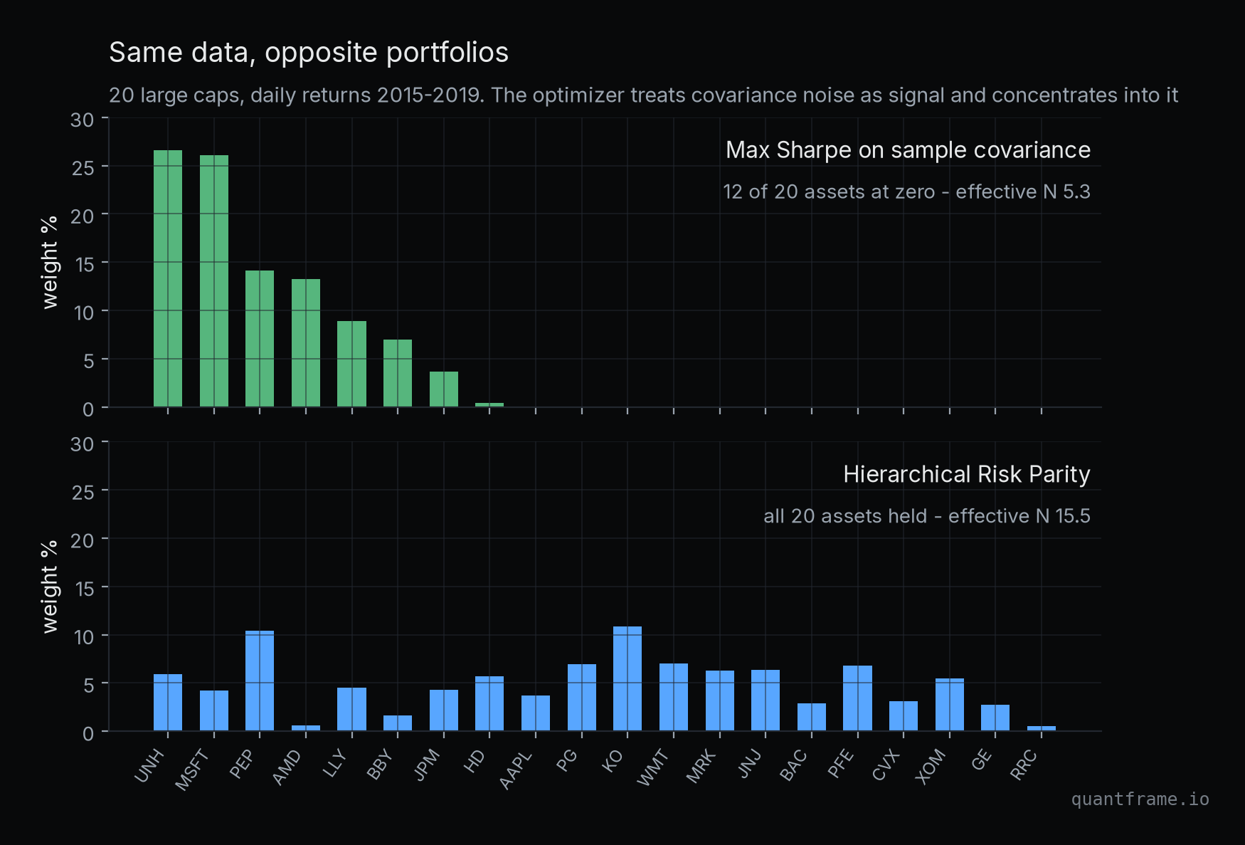
I ran it on skfolio's bundled dataset: 20 large caps, daily returns, fitted on 2015 to 2019. Max Sharpe on the sample covariance put 12 of the 20 assets at exactly zero, 26.6 percent of the book into a single name, and an effective diversification of 5.3 names. Hierarchical Risk Parity on the same data held all 20, capped out at 10.9 percent, effective diversification 15.5.

Two bar panels comparing portfolio weights: max Sharpe on sample covariance concentrates into 8 assets with 12 at zero, while Hierarchical Risk Parity spreads across all 20 — The optimizer's confidence is fake precision. Twelve assets zeroed by max Sharpe are noise judgments, not investment decisions.

Out of sample on 2020 to 2022, the two portfolios earned nearly identical Sharpe ratios, 0.81 against 0.80. Read that carefully: the concentrated portfolio was not smarter, it just took idiosyncratic risk the diversified one refused, and this particular window forgave it. The lesson is fragility, not returns.

skfolio's contribution to the stack is that all of this lives behind the scikit-learn contract: fit, predict, pipelines, walk-forward and combinatorially purged cross-validation. An allocator that is one line to swap is an allocator you can actually test.

NautilusTrader Runs the Loop, skfolio Rides Inside It

NautilusTrader is the execution layer: a Rust core driving an event loop, with strategy logic in Python. Nanosecond-resolution clock, order management, venue adapters, pre-trade risk checks. The one promise the whole architecture bends around: the identical strategy code runs in backtest and live. The backtest replays events in order against a simulated exchange instead of stepping bar by bar, so going live is a config change, not a rewrite.

It is also the slot where most stack articles recommend dead software. Zipline's last release was October 2020, the year Quantopian shut down. Backtrader last shipped in April 2023. Nautilus shipped 1.231.0 in August 2026 with signed releases, SLSA build provenance and an OpenSSF scorecard, which is supply-chain hygiene most trading tools do not bother with.

Here is the actual glue, condensed from the working strategy. skfolio is fitted inside the event loop, on a trailing window the strategy maintains itself:

strategy.pypython

class SkfolioRebalance(Strategy):
    def on_bar(self, bar):
        iid = bar.bar_type.instrument_id
        self.closes[iid].append((bar.ts_event, float(bar.close)))
        if iid != self.bar_types[-1].instrument_id:
            return                       # act once per day, after the last symbol
        self.bar_count += 1
        equity = self.cash() + self.market_value()
        self.psp_equity.update([{"date": self.day(bar), "equity": equity}])
        if self.bar_count % 21 == 0 and self.warmed_up():
            self.rebalance(equity)

    def rebalance(self, equity):
        rets = self.trailing_prices().pct_change().dropna()
        model = HierarchicalRiskParity()
        model.fit(rets)                  # skfolio, inside the event loop
        weights = dict(zip(rets.columns, model.weights_))
        deltas = self.target_deltas(weights, equity)
        deltas.sort(key=lambda x: x[1])  # sells first: they free the cash buys need
        for iid, delta in deltas:
            self.submit_order(self.order_factory.market(
                instrument_id=iid,
                order_side=OrderSide.BUY if delta > 0 else OrderSide.SELL,
                quantity=self.cache.instrument(iid).make_qty(abs(delta)),
            ))

Two seams I hit, so you do not have to rediscover them. Nautilus's bar wrangler currently chokes on pandas 3, because pandas 3 hands out read-only arrays under copy-on-write and the wrangler wants writable memory; constructing Bar objects directly in a 12-line loop sidesteps it. And on a cash account your equity is cash plus position value, which is exactly why the sells-first sort exists: submit buys before the sells clear and the simulated exchange rejects them for insufficient funds, just like a real one would.

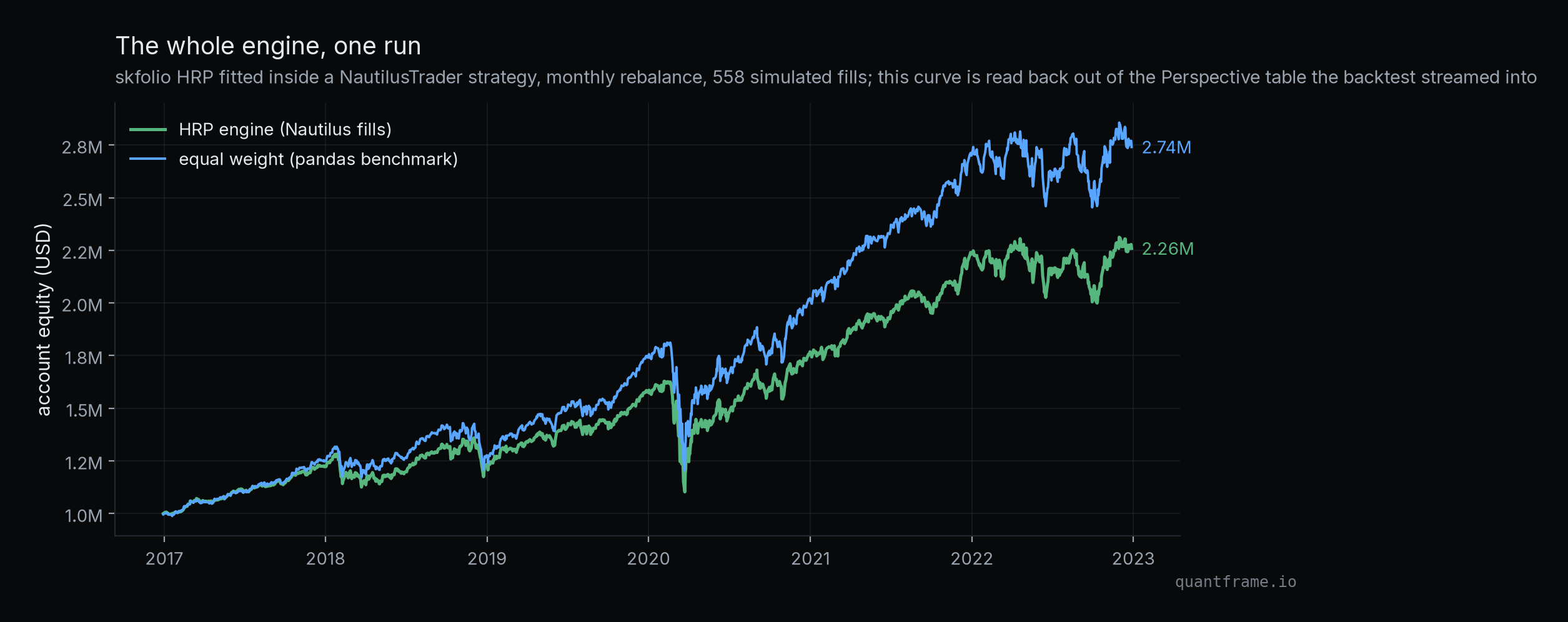
The run: eight US large caps, daily bars 2016 to 2022, monthly HRP rebalance, 1 million USD start. The engine made 558 fills and turned 1M into 2.26M from its first fill in December 2016, a 14.6 percent CAGR with a 32.3 percent max drawdown through the 2020 crash and the 2022 bear.

Equity curves 2017 to 2022: the HRP engine reaching 2.26M USD via NautilusTrader fills versus an equal weight pandas benchmark reaching 2.74M — Both curves survived 2020 and 2022. The green one was produced by orders, fills and an account; the blue one by a pandas one-liner that cannot reject a trade.

And the honest benchmark: naive equal weight over the same window ended at 2.74M with a nearly identical drawdown. HRP loads up on the quiet assets, and in a decade where the loud assets won, that discipline cost return. I am fine publishing that, because the point of this build is the loop, and the allocator is one line to swap. If anything, it is a live demonstration of the skfolio section: diversification logic is a risk decision, not a return promise.

Perspective Is the Only Wire You Can See

Everything so far runs headless. Perspective is where the engine grows a face.

The design is unusual and worth understanding. The same streaming query engine (about 80,000 lines of C++ at the time J.P. Morgan open-sourced it) runs on both sides of the wire: compiled to WebAssembly in the browser, native in the Python server. Your server holds the tables; the browser holds a viewer; instructions travel over a websocket and only results come back. That is why it pivots and filters millions of live rows where an ordinary JavaScript grid dies.

The wire from the trading engine is embarrassingly small. Two tables, and an update call inside the strategy's event handlers:

dashboard_server.pypython

from perspective import Server
from perspective.handlers.tornado import PerspectiveTornadoHandler

server = Server()
client = server.new_local_client()
positions = client.table(
    {"symbol": "string", "qty": "float", "last": "float", "value": "float"},
    index="symbol", name="positions",     # index -> updates overwrite in place
)
equity = client.table({"date": "string", "equity": "float"},
                      index="date", name="equity")

app = tornado.web.Application([
    (r"/ws", PerspectiveTornadoHandler, {"perspective_server": server}),
])

Because the positions table is indexed by symbol, every update from the strategy is an in-place tick, not an append: eight rows that stay eight rows while their values move. The browser side is four lines of JavaScript: open the websocket, open_table("positions"), hand it to a <perspective-viewer> element, done. Pivots, filters, aggregations all execute server-side against live data.

I did not mock this. The backtest above streamed every daily equity point and position snapshot into those tables while it ran, and the equity curve in the last figure was read back out of the Perspective table afterwards, not out of the backtest engine. The websocket handler accepted connections in the same process. The dashboard wire is real.

One warning that Perspective's own source code gives you and most tutorials skip: the bundled handler ships with no authentication at all. It says so in its docstring. On localhost, for you, it is perfect. Exposed to a network, it is an open door to your book.

What a Laptop Engine Is, and What It Is Not

The demo backtest uses close-only daily bars, no transaction costs, no slippage model, and a 98 percent investment cap as its only realism concession. The exposure run prices one swap against one counterparty on a 2016 market snapshot that ships with ORE's examples. Nobody should confuse this with a production system, and the previous article in this series covered what separates a stack from a fund: legal structure, audited capital, and data licensing that costs more per year than every repo here combined, forever, at zero.

What you cannot dismiss is the separation of concerns. Pricing, risk, sizing, execution and display as five independent components with explicit contracts between them is not a toy architecture. It is the same shape a systematic desk runs, and these five repos are the first time every seat in it has a serious open-source occupant. The wires took me about 150 lines of Python. The understanding they forced is the actual product.

What This Means For You

1. Learn the contracts, not the libraries. Returns to weights, weights to orders, positions to risk, state to screen. Every systematic shop on earth is a variation on those four wires. Build them once yourself and every fund's architecture diagram becomes readable.

2. Let the risk number be a different program than the trading number. The industry separates execution from risk on purpose: different code, different assumptions, different failure modes. ORE reading a portfolio file that your execution engine wrote is a healthier design than one program marking its own homework.

3. Version skew is the tax on gluing serious software. Both of my failures (a renamed pricing engine, a pandas 3 memory change) were version mismatches between components that each work perfectly alone. Budget for this. The skill of reading someone else's structured error log is worth more than any single library.

4. Distrust any optimizer that acts certain. Twelve of twenty assets zeroed on five years of daily data is not conviction, it is amplified noise. Prefer allocators that are humble by construction, and always check what a naive benchmark did to your clever one.

5. Demand backtest-live parity from your execution layer. If going live means rewriting the strategy, you have two systems and one of them is untested. This single requirement kills most of the graveyard frameworks and is the strongest reason Nautilus holds its slot.

Every mathematical idea this engine leans on, curve bootstrapping, Monte Carlo exposure, covariance estimation, portfolio construction, is something you can learn by building it. That is exactly what QuantFrame teaches: interactive math, browser-run coding problems, and projects where you implement the real thing. Your personalized roadmap is at quantframe.io.