Search "top quant Python libraries" and you'll get the same list every time. Pandas. NumPy. yfinance. A few mostly-abandoned wrappers around someone's PhD thesis. None of them actually do the math.
Strip away the jargon and quant finance is a small number of hard mathematical problems. You're solving differential equations. You're solving optimization problems. You're doing Bayesian inference over latent state. You're pricing derivatives. That's most of the work. Pick a real research paper from a derivatives desk, an HFT shop, or a systematic fund and you'll see one of these four problems sitting underneath it.
This article is about the five Python libraries that handle those problems seriously. Not toys. Not 50-line wrappers. The libraries that production quants actually use when they need to ship.
Diffrax for stochastic differential equations, with reverse-mode autodiff through the solver.
py-pde for finite-difference PDEs with symbolic equation specification and numba JIT.
CVXPY for convex optimization, all the way up to mixed-integer quadratic programs.
NumPyro for Bayesian inference with NUTS, JAX-compiled, fast enough for real time-series posteriors.
FinancePy for derivatives pricing across equity, rates, FX, and credit, with the models desks actually use.
For each one, I'll show what it is, the problem it solves, and the core code. The visuals in this article are all real output from the libraries themselves. The carousel on Instagram walked through them as a teaser; this is the deep version with code you can actually run.
Setup
Everything below runs in a single Python 3.13 environment. The JAX-based libraries (Diffrax, NumPyro) install CPU JAX by default. CVXPY needs the SCIP backend for the mixed-integer step. py-pde brings numba in as a dep.
Diffrax is a JAX-native library for numerical differential equations, written by Patrick Kidger (the same person who introduced Neural SDEs in his thesis). It covers ODEs, SDEs, and controlled differential equations, and the defining feature is that every solver is reverse-mode autodifferentiable. You can compute exact gradients of the solution with respect to your model parameters by backpropagating through diffeqsolve itself. It composes with jit and vmap and runs identically on CPU, GPU, and TPU.
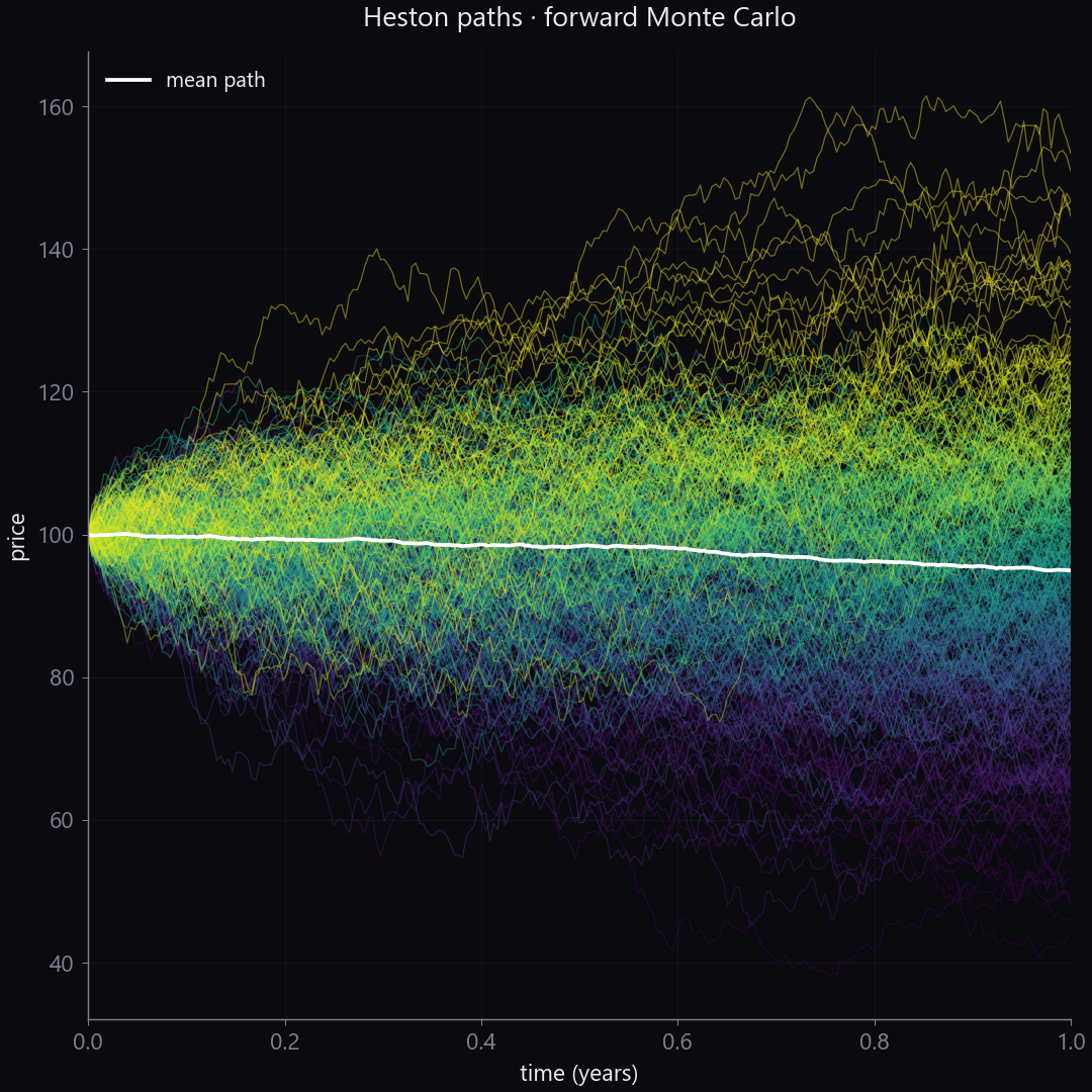
400 Heston paths over T = 1 year. Forward simulation, the easy half.
The problem
The Heston model couples a risk-neutral price St to a mean-reverting instantaneous variance vt:
with correlated drivers ⟨dWS,dWv⟩=ρdt. There are two things you want to do with this model. The first is the forward problem: simulate paths, take expectations, price an option as
C(Θ)=e−rTE[(ST−K)+],Θ=(κ,vˉ,ξ,ρ).
That part every quant library can do. Here it is in Diffrax:
The second thing you want to do is calibrate: given a quoted strike chain {Ckmkt}, find the parameters Θ⋆ that minimize the model-market squared error,
Θ⋆=argΘmink∑(Ckmodel(Θ)−Ckmkt)2.
For gradient-based calibration you need ∇ΘC. Finite differences re-price the chain twice per parameter and the gradient gets dominated by Monte-Carlo variance, so calibration becomes flaky and slow. Characteristic-function pricing works for Heston specifically but doesn't generalize to rough volatility, jumps, or any model where you can't write the MGF in closed form.
Diffrax computes the gradient exactly by backpropagating through the SDE solver itself. The same price function below is differentiated with jax.grad, then optimized with optax.adam.
heston_calibrate.pypython
import jax, jax.numpy as jnp, jax.random as jr
import diffrax as dfx
import optax

S0, v0, r, T = 100.0, 0.04, 0.0, 1.0
kappa, vbar = 2.0, 0.04
xi_true, rho_true = 0.30, -0.70
strikes = jnp.array([90.0, 95.0, 100.0, 105.0, 110.0])
n_paths_c, n_steps_c = 128, 64
KEY = jr.PRNGKey(0)

def price(params, key):
    xi, rho = params
    chol = jnp.array([[1.0, 0.0], [rho, jnp.sqrt(1 - rho ** 2)]])

    def drift(t, y, _):
        return jnp.array([r * y[0], kappa * (vbar - y[1])])

    def diffusion(t, y, _):
        sv = jnp.sqrt(jnp.maximum(y[1], 1e-6))
        return jnp.array([[sv * y[0], 0.0], [0.0, xi * sv]]) @ chol

    def terminal(k):
        bm = dfx.VirtualBrownianTree(0.0, T, tol=1e-3, shape=(2,), key=k)
        terms = dfx.MultiTerm(dfx.ODETerm(drift), dfx.ControlTerm(diffusion, bm))
        return dfx.diffeqsolve(
            terms, dfx.Heun(), 0.0, T, T / n_steps_c,
            jnp.array([S0, v0]),
            saveat=dfx.SaveAt(t1=True),
        ).ys[-1, 0]

    ST = jax.vmap(terminal)(jr.split(key, n_paths_c))
    return jnp.exp(-r * T) * jnp.maximum(ST[:, None] - strikes[None, :], 0.0).mean(0)

# Generate "market" quotes from the true parameters
market = price(jnp.array([xi_true, rho_true]), KEY)

# Loss + gradient -- this is the line that's only possible because
# diffeqsolve is reverse-mode autodifferentiable.
loss      = lambda p: jnp.mean((price(p, KEY) - market) ** 2)
grad_loss = jax.jit(jax.grad(loss))

# Walk from a bad init to the true parameters
params = jnp.array([0.55, 0.40])
opt    = optax.adam(0.04)
state  = opt.init(params)
for _ in range(140):
    updates, state = opt.update(grad_loss(params), state)
    params = optax.apply_updates(params, updates)
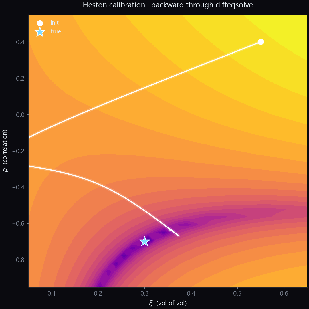
Same Heston model, the backward pass. The white trajectory is adam descending the calibration loss surface, gradients backpropagated through the entire Monte-Carlo SDE pricer. The cyan star is the true (xi, rho).
The second image is what Diffrax was built to enable. Gradient-based calibration of an SDE model with no finite differences and no model-specific Fourier shortcut. Swap the Heston dynamics for rough Bergomi or a jump-diffusion and the calibration code is the same.
2. py-pde: finite-difference PDEs in pure Python
py-pde is a finite-difference PDE solver written in Python with a numba-compiled hot loop. The standout feature is the PDE class. You write the evolution equation as a string in mathematical notation, the library parses it, and numba compiles a fast solver. It supports coupled multi-field systems, custom and time-dependent boundary conditions, stochastic PDEs (SPDEs via SDEBase), and 2D/3D grids in Cartesian, polar, cylindrical, and spherical geometries.
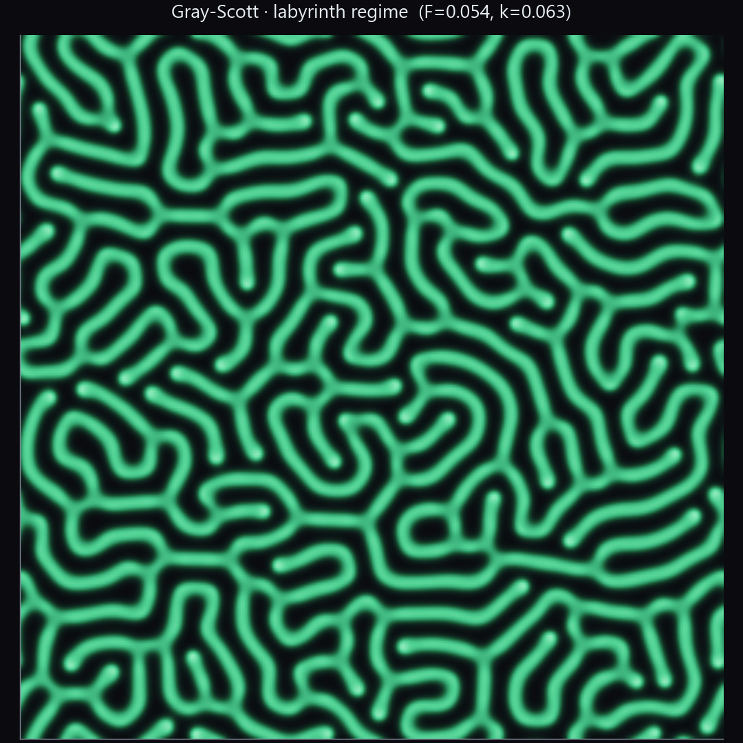
Gray-Scott reaction-diffusion in the labyrinth regime, F = 0.054, k = 0.063. Five seed patches grow into a connected network of filaments.
The problem
Two species u and v diffuse and react on a periodic 2D plane:
∂tu=Du∇2u−uv2+F(1−u),∂tv=Dv∇2v+uv2−(F+k)v.
F feeds species u from a reservoir; k removes species v. For certain regions of the (F,k) plane, a uniform mixture is Turing-unstable: tiny perturbations grow into self-replicating spots, stripes, or labyrinths. The parameters used here, (F,k)=(0.054,0.063), sit in the labyrinthine regime, and the filaments above are the steady state.
This is not finance, but the machinery is. The same finite-difference solver that runs Gray-Scott runs the Black-Scholes PDE backward in time, the Hamilton-Jacobi-Bellman equation for optimal execution, and the Dupire local-volatility equation. The PDE here just happens to be visually extraordinary.
gray_scott.pypython
import numpy as np
from pde import PDE, ScalarField, FieldCollection, UnitGrid, MemoryStorage

N = 256
grid = UnitGrid([N, N], periodic=True)
u, v = ScalarField(grid, 1.0), ScalarField(grid, 0.0)

# Multi-point nucleation: five seed patches with a noisy perturbation.
rng = np.random.default_rng(0)
for cx, cy in [(64, 64), (192, 64), (64, 192), (192, 192), (128, 128)]:
    u.data[cy-10:cy+10, cx-10:cx+10] = 0.50
    v.data[cy-10:cy+10, cx-10:cx+10] = 0.25
v.data = np.maximum(v.data + 0.02 * rng.standard_normal(grid.shape), 0.0)
state = FieldCollection([u, v])

# This is the entire solver. Symbolic specification, numba compiles the rest.
eq = PDE(
    {
        "u": "Du * laplace(u) - u * v**2 + F * (1 - u)",
        "v": "Dv * laplace(v) + u * v**2 - (F + kk) * v",
    },
    consts={"Du": 0.16, "Dv": 0.08, "F": 0.054, "kk": 0.063},
)

storage = MemoryStorage()
result = eq.solve(state, t_range=15000, dt=1.0, tracker=storage.tracker(60))
Five lines specify the PDE, one line solves it, the MemoryStorage tracker stores intermediate frames so you can render the evolution as an animation. A from-scratch numpy port is fast to write but roughly 10x slower at runtime, and you'd reinvent the storage and animation pipeline yourself.
3. CVXPY: convex optimization as a DSL
CVXPY is a domain-specific language for convex optimization, developed by Stephen Boyd's group at Stanford. You write the problem in math notation, the library verifies convexity through the Disciplined Convex Programming (DCP) ruleset, transforms it into standard cone form, and dispatches it to a solver. It covers LP, QP, SOCP, SDP, MILP, MIQP, robust optimization, and chance constraints in the same syntax. The solver list is plug-and-play: ECOS, SCS, OSQP, CLARABEL, SCIP, CBC, plus the commercial ones (GUROBI, MOSEK).
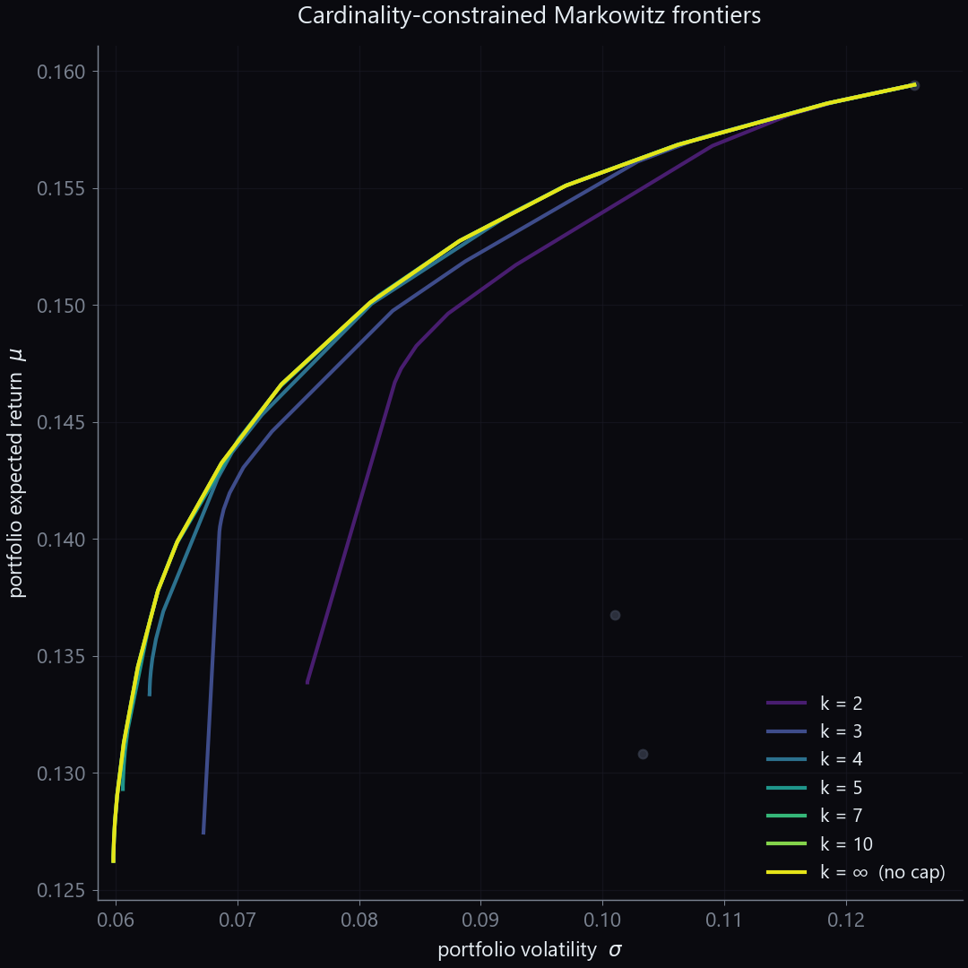
Seven Markowitz efficient frontiers under a 'hold at most k positions' constraint. The curves for k >= 5 collapse onto the unconstrained frontier; sparsity stops costing Sharpe once you allow about five names.
The problem
Classical mean-variance portfolio selection picks weights w∈Rn to trade off expected return against variance:
wmin21w⊤Σws.t.μ⊤w≥rtgt,1⊤w=1,w≥0.
That's a quadratic program. Three lines in CVXPY, solved in milliseconds.
Real portfolios face an additional operational, tax, or regulatory constraint: hold at most k non-zero positions. Adding ∥w∥0≤k turns the QP into a mixed-integer quadratic program (MIQP), enforced through binary indicators z∈{0,1}n with wi≤zi and ∑zi≤k.
What CVXPY lets you do is add the integer constraint by changing one keyword. Same problem object, same solve call, the library re-dispatches to SCIP under the hood.
markowitz_miqp.pypython
import numpy as np
import cvxpy as cp

# 30-asset universe: 6 sectors of 5, block correlation structure.
rng = np.random.default_rng(7)
n = 30
mu     = 0.03 + 0.13 * rng.uniform(size=n)
sigmas = 0.10 + 0.28 * rng.uniform(size=n)
sector = np.repeat(np.arange(6), 5)
corr   = np.where(sector[:, None] == sector[None, :], 0.65, 0.10)
np.fill_diagonal(corr, 1.0)
Sigma  = np.outer(sigmas, sigmas) * corr

def cardinality_frontier(k, n_pts=24):
    w   = cp.Variable(n, nonneg=True)
    z   = cp.Variable(n, boolean=True)         # <-- this single keyword turns QP into MIQP
    lam = cp.Parameter(nonneg=True)
    obj = cp.Minimize(lam * cp.quad_form(w, cp.psd_wrap(Sigma)) - mu @ w)
    prob = cp.Problem(obj, [cp.sum(w) == 1, w <= z, cp.sum(z) <= k])

    points = []
    for l in np.logspace(-1.5, 2.5, n_pts):
        lam.value = float(l)
        prob.solve(solver="SCIP")
        if prob.status == "optimal":
            vol = float(np.sqrt(w.value @ Sigma @ w.value))
            ret = float(mu @ w.value)
            points.append((vol, ret))
    return np.array(sorted(set(points)))

frontiers = {k: cardinality_frontier(k) for k in [2, 3, 4, 5, 7, 10, 30]}
The story the visual tells: at k=2 the frontier sits well inside the unconstrained one, at k=3 slightly less so, and by k=5 the curve has essentially caught up. The cardinality constraint stops binding around five names for this universe. Translation: you can hold a 30-stock universe with five concentrated positions and lose almost no Sharpe. Going to three costs real return at every risk level. Going to two is a serious haircut.
The whole optimization is about thirteen lines. Re-implementing this against a raw MIQP solver (Gurobi's Python API, say) is five times the code and pinned to one backend.
4. NumPyro: gradient-based MCMC for real time-series posteriors
NumPyro is a JAX-backed probabilistic programming language. You write a generative model with numpyro.sample(...) statements and numpyro.contrib.control_flow.scan for time-series; NumPyro gives you the No-U-Turn variant of HMC (NUTS, the adaptive-trajectory sampler that powers most modern Bayesian inference) plus variational inference (SVI) and a large distributions library. NUTS through JAX autodiff is one of the fastest mainstream gradient-based MCMC implementations available.
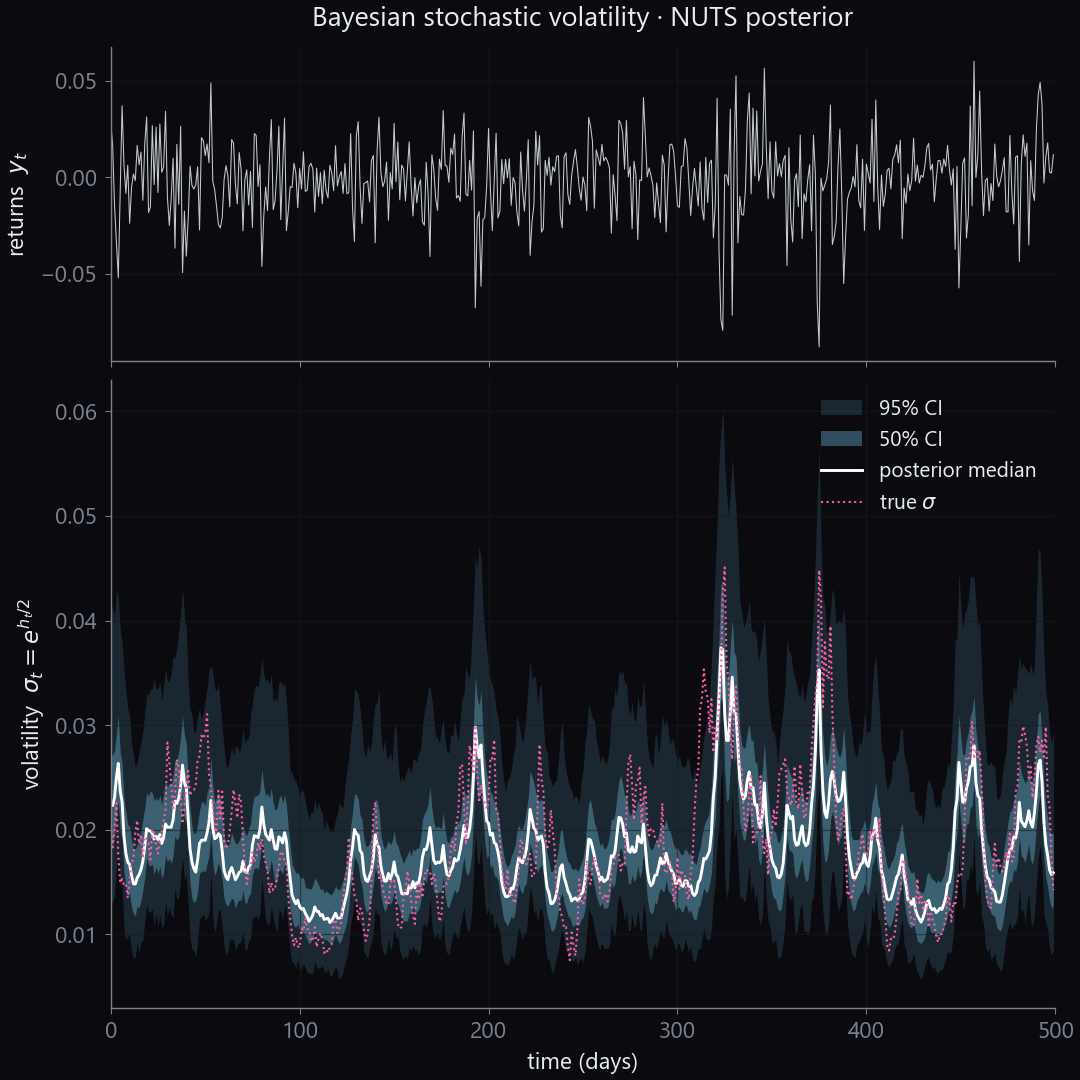
Top: 500 days of simulated returns. Bottom: posterior over the latent volatility path inferred by NUTS, with 50 and 95 percent credible bands, true volatility dashed. The full posterior is 503-dimensional and the sampler clears it in about a minute.
The problem
A latent log-variance ht follows an AR(1) process, and conditional on ht the returns yt are Gaussian with time-varying scale:
ht=μ+ϕ(ht−1−μ)+σηηt,yt=exp(ht/2)ϵt.
The inference target is the joint posterior p(μ,ϕ,ση,h∣y) over both the structural parameters and the full latent volatility path h=(h1,…,hT). For T=500 that's a 503-dimensional posterior with very strong correlations between consecutive ht. Random-walk samplers stall on this geometry. NUTS uses the gradient of the log-posterior with respect to all 503 latent variables to pick its step direction, and JAX provides that gradient through autodiff.
sv_model.pypython
import jax, jax.numpy as jnp
import numpy as np
import numpyro
import numpyro.distributions as dist
from numpyro.infer import MCMC, NUTS
from numpyro.contrib.control_flow import scan

# Synthetic ground truth: 500 days of returns generated by an AR(1) log-vol.
T = 500
mu_t, phi_t, sig_t = -8.0, 0.96, 0.25
rng = np.random.default_rng(42)
h_true = np.zeros(T)
h_true[0] = mu_t + sig_t * rng.standard_normal() / np.sqrt(1 - phi_t ** 2)
for t in range(1, T):
    h_true[t] = mu_t + phi_t * (h_true[t - 1] - mu_t) + sig_t * rng.standard_normal()
y = np.exp(h_true / 2) * rng.standard_normal(T)

# The entire model: 11 lines. Priors on the structural parameters, then a
# scan over the latent volatility path, then the observation likelihood.
def sv_model(y):
    mu        = numpyro.sample("mu",        dist.Normal(-8.0, 2.0))
    phi       = numpyro.sample("phi",       dist.Uniform(0.0, 0.999))
    sigma_eta = numpyro.sample("sigma_eta", dist.HalfNormal(0.5))

    h0 = numpyro.sample("h_0", dist.Normal(mu, sigma_eta / jnp.sqrt(1 - phi ** 2)))

    def step(h_prev, _):
        h = numpyro.sample("h", dist.Normal(mu + phi * (h_prev - mu), sigma_eta))
        return h, h

    _, h = scan(step, h0, jnp.arange(len(y)))
    numpyro.sample("y", dist.Normal(0.0, jnp.exp(h / 2)), obs=y)

mcmc = MCMC(NUTS(sv_model), num_warmup=600, num_samples=1000, progress_bar=False)
mcmc.run(jax.random.PRNGKey(0), y=jnp.asarray(y))
samples = mcmc.get_samples()      # samples["h"] has shape (1000, 500)
The same autodiff machinery that backpropagates through diffeqsolve in section 1 lets NUTS compute the gradient of the log-posterior with respect to all 503 latent variables in a single backward pass. That gradient is what tells the sampler which way to move. Stan does the same thing but in its own language. PyMC does it about 5x slower for high-dim time-series posteriors. For Bayesian SV models, NumPyro is the live option.
5. FinancePy: derivatives pricing and the models desks actually trade
FinancePy is a pure-Python derivatives pricing and risk library by Dominic O'Kane (ex-Lehman, now NYU). The coverage is broad. Equity options, fixed income, FX, credit, inflation, structured products. And it ships with the models that desks actually use: Black-Scholes, Heston, SABR, Bachelier, Hull-White, LMM. Pricing methods include closed-form (Heston via characteristic function), Monte Carlo, PDE, and tree-based. The library bootstraps yield curves and fits implied vol surfaces out of the box.
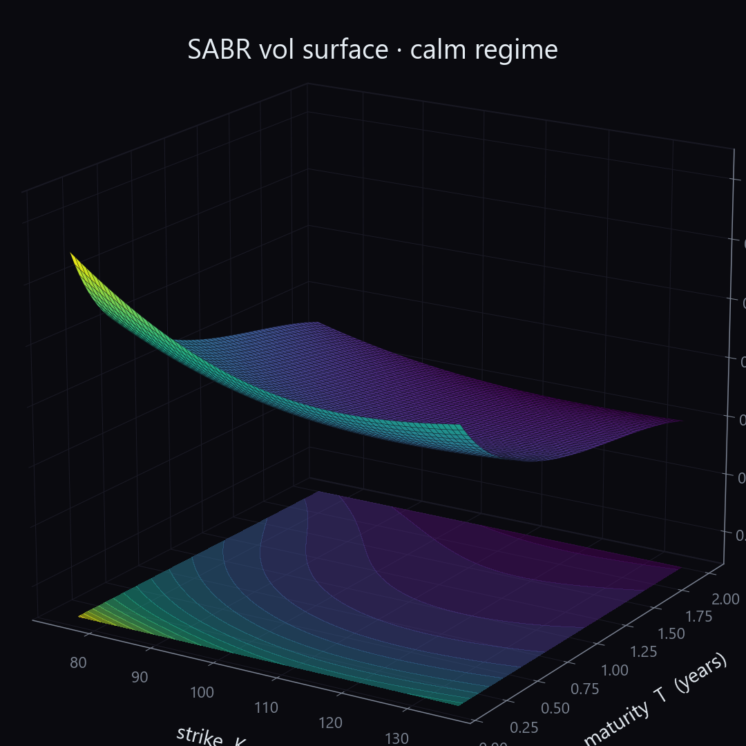
SABR vol surface fitted to a calm regime. Mild skew, low vol of vol, nearly flat ATM term structure.
The problem
SABR (Hagan et al., 2002) parameterizes the implied-volatility surface through four parameters (α,β,ρ,ν). Under the SABR dynamics
dFt=σtFtβdWtF,dσt=νσtdWtσ,⟨dWF,dWσ⟩=ρdt,
Hagan's asymptotic expansion gives a closed-form Black implied volatility σBS(K,T;α,β,ρ,ν,F). Fast enough to calibrate a smile in milliseconds. With β fixed at 1 (lognormal SABR), each maturity slice has three free parameters: α for the ATM vol level, ρ for the skew, ν for the vol of vol.
Implementing the Hagan formula from the paper is about 50 lines including edge cases (the ATM limit, β=0 and β=1 branches, near-money handling). FinancePy gives you the same thing, debugged and tested, in one line.
sabr_surface.pypython
import numpy as np
from scipy.interpolate import interp1d
from financepy.models.sabr import SABR

F     = 100.0
beta  = 1.0
maturities = [0.10, 0.25, 0.50, 1.00, 2.00]

# (alpha, rho, nu) per maturity for two market regimes.
calm_params = [
    (0.16, -0.30, 0.45),
    (0.15, -0.27, 0.36),
    (0.14, -0.25, 0.30),
    (0.13, -0.22, 0.25),
    (0.12, -0.20, 0.20),
]
stressed_params = [
    (0.42, -0.78, 1.70),
    (0.38, -0.72, 1.25),
    (0.34, -0.66, 0.95),
    (0.30, -0.60, 0.75),
    (0.26, -0.55, 0.60),
]

def build_surface(params_list):
    # Smoothly interpolate the calibrated SABR params through maturity.
    alpha_fn = interp1d(maturities, [p[0] for p in params_list], kind="cubic")
    rho_fn   = interp1d(maturities, [p[1] for p in params_list], kind="cubic")
    nu_fn    = interp1d(maturities, [p[2] for p in params_list], kind="cubic")

    K_arr   = np.linspace(75, 135, 70)
    T_arr   = np.linspace(0.10, 2.00, 60)
    K_grid, T_grid = np.meshgrid(K_arr, T_arr)
    IV_grid = np.zeros_like(K_grid)
    for i, Tm in enumerate(T_arr):
        m = SABR(float(alpha_fn(Tm)), beta, float(rho_fn(Tm)), float(nu_fn(Tm)))
        for j, K in enumerate(K_arr):
            IV_grid[i, j] = m.black_vol(F, K, Tm)
    return K_grid, T_grid, IV_grid

calm_K,    calm_T,    calm_IV    = build_surface(calm_params)
stress_K,  stress_T,  stress_IV  = build_surface(stressed_params)
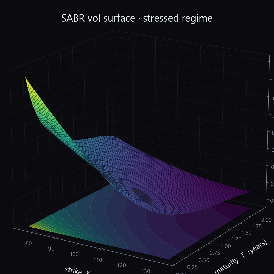
Same parameterization, stressed regime. Sharp negative skew, large vol of vol, steep ramp into the downside-strike corner. This is what a desk sees during a crisis.
Two states of the same model, rendered on the same axes. ATM vol decreases with maturity in both (the surface flattens going back). The smile is steepest at short maturity (steep ramp on the left at T→0). Skew is negative throughout, sharply so in the stressed regime. These are the features every options desk monitors. SABR is also the model that actually trades on every interest-rate, FX, and equity-vol desk worldwide. FinancePy's SABR(alpha, beta, rho, nu).black_vol(F, K, T) is one line.
Note the connection back to section 1. The Diffrax visual fit Heston by backpropagating through a Monte Carlo SDE solver. This visual fits SABR using a closed-form expansion plus scipy.optimize.minimize. Same fundamental problem (calibrate a vol model to market quotes), two completely different solver paths, two different libraries. Both are how it really gets done.
Putting the toolkit together
If you took every quant paper published in the last five years and looked at the libraries actually used, this is most of what you'd see, with PyTorch occupying the rest of the JAX share for ML-heavy work. The five solve four different problems:
Differential equations, including stochastic ones, where the model parameters need calibration. Diffrax.
Convex optimization with portfolio constraints, hedging, execution, risk budgeting. CVXPY.
Bayesian inference over latent state in a non-trivial geometry. NumPyro.
Derivatives pricing with the standard models, calibration utilities, and risk metrics. FinancePy.
Real workflows use them in combination. A research desk might calibrate Heston with Diffrax (because they want to extend to a rough-volatility model where Fourier methods fail), price the calibrated model with FinancePy's analytic Heston implementation for sanity checks, then run portfolio-level risk through CVXPY. None of these libraries are toys, and none of them are doing what NumPy alone can do.
That's the deep version of the carousel. If you want more of this kind of breakdown, with code and visuals from real libraries, follow along on Instagram. The next one is already in progress.
End of entry
Found this useful?
Likes decide what gets written next.Sign in to like
QuantFrame
Liked this article?
QuantFrame teaches you the math, code, and projects to break into quant. Plus a personalized roadmap built for your background and goals.